This repository has been archived by the owner on Dec 15, 2021. It is now read-only.
-
Notifications
You must be signed in to change notification settings - Fork 21
/
lukavdplas - Ellipses.jl
383 lines (289 loc) · 12.8 KB
/
lukavdplas - Ellipses.jl
1
2
3
4
5
6
7
8
9
10
11
12
13
14
15
16
17
18
19
20
21
22
23
24
25
26
27
28
29
30
31
32
33
34
35
36
37
38
39
40
41
42
43
44
45
46
47
48
49
50
51
52
53
54
55
56
57
58
59
60
61
62
63
64
65
66
67
68
69
70
71
72
73
74
75
76
77
78
79
80
81
82
83
84
85
86
87
88
89
90
91
92
93
94
95
96
97
98
99
100
101
102
103
104
105
106
107
108
109
110
111
112
113
114
115
116
117
118
119
120
121
122
123
124
125
126
127
128
129
130
131
132
133
134
135
136
137
138
139
140
141
142
143
144
145
146
147
148
149
150
151
152
153
154
155
156
157
158
159
160
161
162
163
164
165
166
167
168
169
170
171
172
173
174
175
176
177
178
179
180
181
182
183
184
185
186
187
188
189
190
191
192
193
194
195
196
197
198
199
200
201
202
203
204
205
206
207
208
209
210
211
212
213
214
215
216
217
218
219
220
221
222
223
224
225
226
227
228
229
230
231
232
233
234
235
236
237
238
239
240
241
242
243
244
245
246
247
248
249
250
251
252
253
254
255
256
257
258
259
260
261
262
263
264
265
266
267
268
269
270
271
272
273
274
275
276
277
278
279
280
281
282
283
284
285
286
287
288
289
290
291
292
293
294
295
296
297
298
299
300
301
302
303
304
305
306
307
308
309
310
311
312
313
314
315
316
317
318
319
320
321
322
323
324
325
326
327
328
329
330
331
332
333
334
335
336
337
338
339
340
341
342
343
344
345
346
347
348
349
350
351
352
353
354
355
356
357
358
359
360
361
362
363
364
365
366
367
368
369
370
371
372
373
374
375
376
377
378
379
380
381
382
383
### A Pluto.jl notebook ###
# v0.14.0
using Markdown
using InteractiveUtils
# This Pluto notebook uses @bind for interactivity. When running this notebook outside of Pluto, the following 'mock version' of @bind gives bound variables a default value (instead of an error).
macro bind(def, element)
quote
local el = $(esc(element))
global $(esc(def)) = Core.applicable(Base.get, el) ? Base.get(el) : missing
el
end
end
# ╔═╡ 41038420-032c-11eb-3351-d3b98b982502
begin
import Pkg
Pkg.activate(mktempdir())
Pkg.add([
Pkg.PackageSpec(name="Plots")
])
using Plots
end
# ╔═╡ 51f23aae-0946-11eb-1bab-93dcbc98f564
md"""
# The circumference of an ellipse
This notebook is inspired by [Matt Parker's video](https://youtu.be/5nW3nJhBHL0) on the same topic. Notebook by [Luka van der Plas](https://github.com/lukavdplas).
You are (hopefully) familiar with the formula to calculate the circumference of a circle. If we have a circle with radius $r$...
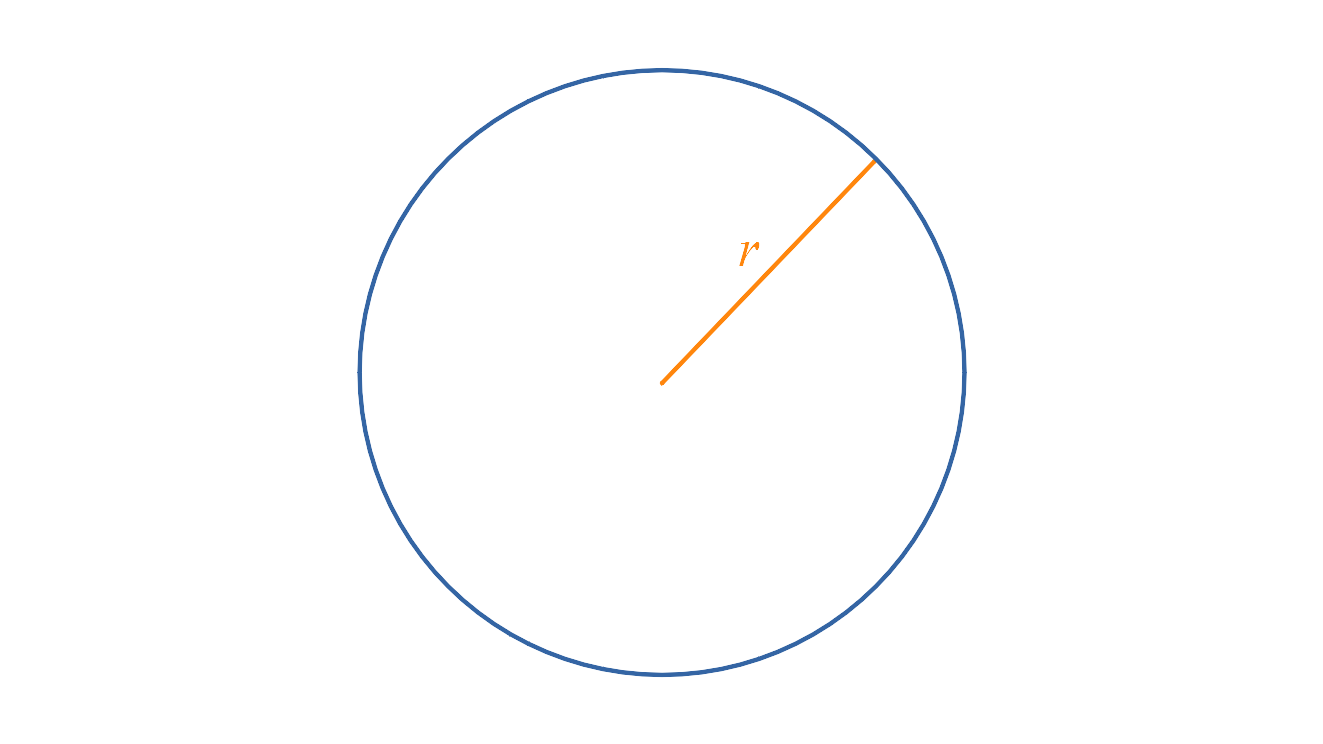
... then the circumference $C$ is equal to $2πr$.
**But what is the formula for an ellipse?**
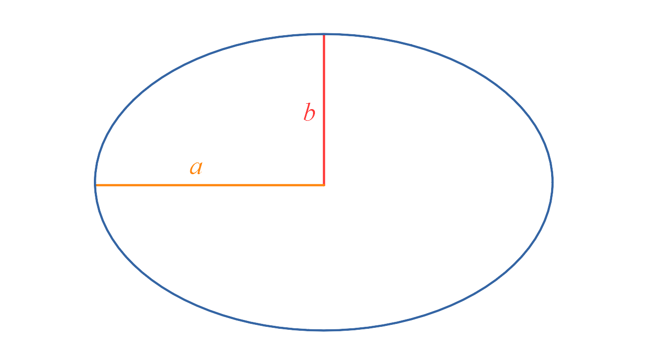
Because an ellipse is elongated, we can't just describe it with a single value for the radius. Instead, we give the _semi-major axis_, $a$, and the _semi-minor axis_, $b$.
(The _semi-_bit means that we go form the centre to the edge, not from one edge to the other. So $a$ and $b$ are analogous to the radius, not the diameter.)
Let's start by making a structure for that.
"""
# ╔═╡ 548569a6-032b-11eb-33cc-af77acc58e4c
struct Ellipse
a
b
#constructors
Ellipse(a,b) = a >= b ? new(a,b) : error("a must be the larger axis")
Ellipse(a) = a >= 1 ? new(a, 1) : error("a must be the larger axis")
end
# ╔═╡ 90970ddc-0948-11eb-24c8-43daa4717fc8
md"""
Our `Ellipse` struct stores the valus of $a$ and $b$. I also defined some constructors. If you give the values of $a$ and $b$, the constructor will check if $a$ is not smaller than $b$, and give you an error otherwise.
You can also make an ellipse by just given a value for $a$. We then assume that $b = 1$.
Okay, let's make an ellipse!
"""
# ╔═╡ 6b494aa4-032b-11eb-1a88-e15df14a934f
shape = Ellipse(2)
# ╔═╡ 27b372fa-0949-11eb-15a0-1f5c41dec2f3
md"""
You can retrieve the values of the axes by putting `.a` or `.b` behind the name.
"""
# ╔═╡ 46298274-0949-11eb-3c9b-654a1fb92cbe
shape.a
# ╔═╡ 496da6f4-0949-11eb-3e5c-73278ab92860
shape.b
# ╔═╡ 9c36f9cc-04b1-11eb-3174-0390e0e731a8
md"""
These values are really all we need to do some geometry. But it's probably nice to have some visualisation as well. Here is a picture of our ellipse:
"""
# ╔═╡ b171c514-0949-11eb-01aa-1f7d5f3470ca
md"""
Beautiful.
Now, let's go back to our question: how do we calculate the circumference of an ellipse?
Surprisingly, there is no neat formula! There are some infinite series, but those are not exactly easy to use. For example, we can calculate the circumference $C$ using the following formula:
$C = \pi (a + b) \bigg( 1 + \sum_{n = 1}^\infty \Big( \frac{(2n - 1)!!}{2^n n!} \Big) ^2 \frac{h^n}{(2n -1)^2} \bigg)$
where
$h = \frac{(a - b)^2}{(a + b)^2}$
Oof.
Don't worry about understanding the formula. One thing of note: the formula contains an infinite sum (note the $∞$ sign above the $\Sigma$). We can't actually repeat a calculation into infinity, but the more steps we make, the closer the result will be to the actual circumference. In fact, for any level of precision that we want, we can find a number of steps that will guarantee that precision.
This formula is a hassle to encode in a Julia in the 21st century. (Don't worry, I already did that for you.) But using a formula like that was even worse in History Times, when people did not have computers at their disposal. So instead, people would use approximation functions.
An approximation function will give you something _close_ to the real circumference, but it's easier to calculate. That is what we will do in this notebook! We can encode some functions and compare them to the "true" value of the circumference.
"""
# ╔═╡ 68d34a1c-0953-11eb-1631-0db60515316e
md"""
## Approximations
Let's define some approximation functions. A function should take an ellipse as input, and return the circumference. Here is a simple example:
"""
# ╔═╡ 91f220c6-0953-11eb-0916-975e36ec27ca
function π_a_plus_b(el::Ellipse)
π * (el.a + el.b)
end
# ╔═╡ 48531a3c-0954-11eb-1b36-0b4408fe7c6f
π_a_plus_b(shape)
# ╔═╡ 6841d7f8-04ba-11eb-0553-2d898d29bbc1
md"""
To compare these functions, we will keep them in a `Dict`. This one will store a good name for the function, and the function itself. The names will be useful when we make a plot.
"""
# ╔═╡ 591f43c0-0954-11eb-2008-eb741b0e3b0a
md"""
Some more functions. You can add more your own (see Matt's video for inspiration), or even try to find the best function you can!
(Remember that if you want to add a function to the plot below, you have to include it in the `approximations` dict.)
"""
# ╔═╡ bf052cba-04b8-11eb-271d-a3d2697ebef8
function ramanujan(el::Ellipse)
π * (3 * (el.a + el.b) - sqrt(10*el.a*el.b + 3(el.a^2 + el.b^2)))
end
# ╔═╡ 2da68146-04b9-11eb-1e8d-71ad1a622c4e
function parker(el::Ellipse)
π * (6 * el.a / 5 + 3 * el.b / 4)
end
# ╔═╡ 67a6224e-04b3-11eb-3f32-c75b44d59920
approximations = Dict(
"π(a + b)" => π_a_plus_b,
"Ramanujan" => ramanujan,
"Matt Parker" => parker)
# ╔═╡ 2882c10a-0952-11eb-0258-bfd6310ae6ba
md"""
## Results
This plot shows how all of our functions are doing.
We are interested in the _error_ of our function, i.e. how far it is from the real circumference. In this plot, we compare it to the ratio $\frac{a}{b}$, so we can see how well it does in ellipses with various shapes. If the ratio is 1, we just have a circle. The higher the ratio, the more elongated our ellipse is.
"""
# ╔═╡ 9dcaf956-04ba-11eb-071f-258a3d23037a
md"""
Here are some options for your plot:
"""
# ╔═╡ f5cc3c80-094e-11eb-2cfc-478093f5e915
@bind give_absolute html"<input type=checkbox checked=checked> Give absolute value of error <br> <i>Turn all errors into postive values</i>"
# ╔═╡ 5403bd12-0951-11eb-2eb2-d1b0a703e319
@bind give_relative html"""<input type=checkbox checked=checked> Give error relative to circumference <br> <i>Divide the error by the circumference. Note that you will probably need to adjust the scale as well.</i>"""
# ╔═╡ 56320014-094f-11eb-1642-37841339e58d
md"""
Maximum error:
$(@bind log_max_error html"<input type=range min=-4 max=1 value=-1 step=0.1>")
*What should be the limit on the y axis?*
"""
# ╔═╡ f7a322f6-0952-11eb-2691-f740b6266ac3
md"""
Maximum $\frac{a}{b}$ ratio:
$(@bind max_ratio html"<input type=range min=2 max=20 value=5>")
*What should be the limit on the x-axis?*
"""
# ╔═╡ b0a21d8c-8f5f-46e6-87f0-cca0def156a0
md"""
Number of data points:
$(@bind sample_size html"<input type=range min=5 max=300 value=100>")
*Slide up if you want more precision in the plot, slide down if you want to speed up calculations.*
"""
# ╔═╡ dc7e33a8-094b-11eb-3805-6f3dfc195c75
md"""
## The true circumference
If you are interested, here is the code I used to calculate the "true" circumference and to compare that with the approximations.
Though you probably remember the formula, this is the infinite series we can use to get the true circumference.
$C = \pi (a + b) \bigg( 1 + \sum_{n = 1}^\infty \Big( \frac{(2n - 1)!!}{2^n n!} \Big) ^2 \frac{h^n}{(2n -1)^2} \bigg)$
where
$h = \frac{(a - b)^2}{(a + b)^2}$
As I mentioned, you can sum to a particular value of $n$ to get the level of precision that you want. I used $n = 10$.
"""
# ╔═╡ eb382296-0955-11eb-1b75-f564dca3e7bc
function double_factorial(n)
sequence = (n % 2 == 1) ? (1:2:n) : (2:2:n)
reduce(*, sequence)
end
# ╔═╡ c6afe960-032e-11eb-270f-afceb7ee6ec2
function h(el::Ellipse)
(el.a - el.b)^2 / (el.a + el.b)^2
end
# ╔═╡ b2c6fe54-032f-11eb-3b2e-07fef89c6593
function circumference(el::Ellipse; precision=10)
series = map(1:precision) do n
first_fraction = double_factorial(2n-1) / ((2^n) * factorial(n))
second_faction = h(el)^n / ((2n-1)^2)
first_fraction ^ 2 * second_faction
end
π * (el.a + el.b ) * (1 + sum(series))
end
# ╔═╡ b4595b58-04b1-11eb-2083-7f887d151c2c
circumference(shape)
# ╔═╡ bcdf9f38-0954-11eb-0536-d38e4654ac5d
md"""
To create the plot, we generate a range of values for the $\frac{a}{b}$ ratio and calculate the "true" circumference for each.
"""
# ╔═╡ fbb7be8a-04b2-11eb-2a1d-b54b3b901a6c
test_ratios = range(1,max_ratio, length=sample_size)
# ╔═╡ ed9b7da6-04b4-11eb-3881-6b47fa5e07d5
function true_curve(ratios)
map(ratios) do ratio
el = Ellipse(ratio)
circumference(el)
end
end
# ╔═╡ e9b4c6d6-04b4-11eb-14d0-1902df47b214
circumferences = true_curve(test_ratios)
# ╔═╡ e91f9ee0-0954-11eb-0053-4364fbd5e096
md"""
For a particular approximation function, we can get the errors by applying the function to each ratio, and substracting the true circumference from the result.
"""
# ╔═╡ fe5744c4-04b1-11eb-0631-1de63b183b3e
function error_curve(func, ratios, circs; absolute = true)
guesses = map(ratios) do ratio
el = Ellipse(ratio)
func(el)
end
if absolute
abs.(guesses .- circs)
else
guesses .- circs
end
end
# ╔═╡ 20a38854-0955-11eb-15d9-bd5c5cbc7165
md"""
To get the relative error, we also divide by the circumference.
"""
# ╔═╡ adbc6a96-04b2-11eb-0102-578a46548aed
function relative_error_curve(func, ratios, circs; absolute = true)
errors = error_curve(func, ratios, circs, absolute = absolute)
errors ./ circs
end
# ╔═╡ 3efe96f0-04b3-11eb-2d98-774f7aa7c377
let
lims = if give_absolute
(0, 10.0^log_max_error)
else
(-10.0^log_max_error, 10.0^log_max_error)
end
label = give_relative ? "relative error" : "error"
p = plot(xlabel = "ratio a/b", ylabel = label, ylims = lims)
for name in keys(approximations)
func = approximations[name]
curve = if give_relative
relative_error_curve(func,
test_ratios, circumferences, absolute = give_absolute)
else
error_curve(func, test_ratios, circumferences, absolute = give_absolute)
end
plot!(p, test_ratios, curve,
label = name, lw = 2)
end
p
end
# ╔═╡ 0ff28cba-12e6-11eb-33c3-236317fcb1a6
md"Lastly, here is the function I used to display the ellipse in the beginning."
# ╔═╡ 44ab1d7c-032c-11eb-0d82-bb23901148f3
function show_ellipse(el::Ellipse)
angles = range(0, 4π, length=100)
limits = (- el.a, el.a) .* 1.05
plot(el.a .* sin.(angles), el.b .* cos.(angles), #formula
xlim = limits, ylim = limits, size = (500, 500), #show a/b ratio correctly
lw =3, #linewidth
legend = false, framestyle = :none #hide axes and legend
)
end
# ╔═╡ b7d212b0-032c-11eb-235f-eb2f2b85292c
show_ellipse(shape)
# ╔═╡ Cell order:
# ╟─51f23aae-0946-11eb-1bab-93dcbc98f564
# ╠═548569a6-032b-11eb-33cc-af77acc58e4c
# ╟─90970ddc-0948-11eb-24c8-43daa4717fc8
# ╠═6b494aa4-032b-11eb-1a88-e15df14a934f
# ╟─27b372fa-0949-11eb-15a0-1f5c41dec2f3
# ╠═46298274-0949-11eb-3c9b-654a1fb92cbe
# ╠═496da6f4-0949-11eb-3e5c-73278ab92860
# ╟─9c36f9cc-04b1-11eb-3174-0390e0e731a8
# ╟─b7d212b0-032c-11eb-235f-eb2f2b85292c
# ╟─b171c514-0949-11eb-01aa-1f7d5f3470ca
# ╟─68d34a1c-0953-11eb-1631-0db60515316e
# ╠═91f220c6-0953-11eb-0916-975e36ec27ca
# ╠═48531a3c-0954-11eb-1b36-0b4408fe7c6f
# ╟─6841d7f8-04ba-11eb-0553-2d898d29bbc1
# ╠═67a6224e-04b3-11eb-3f32-c75b44d59920
# ╟─591f43c0-0954-11eb-2008-eb741b0e3b0a
# ╠═bf052cba-04b8-11eb-271d-a3d2697ebef8
# ╠═2da68146-04b9-11eb-1e8d-71ad1a622c4e
# ╟─2882c10a-0952-11eb-0258-bfd6310ae6ba
# ╟─3efe96f0-04b3-11eb-2d98-774f7aa7c377
# ╟─9dcaf956-04ba-11eb-071f-258a3d23037a
# ╟─f5cc3c80-094e-11eb-2cfc-478093f5e915
# ╟─5403bd12-0951-11eb-2eb2-d1b0a703e319
# ╟─56320014-094f-11eb-1642-37841339e58d
# ╟─f7a322f6-0952-11eb-2691-f740b6266ac3
# ╟─b0a21d8c-8f5f-46e6-87f0-cca0def156a0
# ╟─dc7e33a8-094b-11eb-3805-6f3dfc195c75
# ╠═b2c6fe54-032f-11eb-3b2e-07fef89c6593
# ╠═eb382296-0955-11eb-1b75-f564dca3e7bc
# ╠═c6afe960-032e-11eb-270f-afceb7ee6ec2
# ╠═b4595b58-04b1-11eb-2083-7f887d151c2c
# ╟─bcdf9f38-0954-11eb-0536-d38e4654ac5d
# ╠═fbb7be8a-04b2-11eb-2a1d-b54b3b901a6c
# ╠═ed9b7da6-04b4-11eb-3881-6b47fa5e07d5
# ╠═e9b4c6d6-04b4-11eb-14d0-1902df47b214
# ╟─e91f9ee0-0954-11eb-0053-4364fbd5e096
# ╠═fe5744c4-04b1-11eb-0631-1de63b183b3e
# ╟─20a38854-0955-11eb-15d9-bd5c5cbc7165
# ╠═adbc6a96-04b2-11eb-0102-578a46548aed
# ╟─0ff28cba-12e6-11eb-33c3-236317fcb1a6
# ╠═44ab1d7c-032c-11eb-0d82-bb23901148f3
# ╠═41038420-032c-11eb-3351-d3b98b982502