Asteroid Diameter Prediction: EDA

I also recommend reading the notebook on Kaggle.

SUMMARY

• Developed an innovative approximate diameter feature in the MLP model, resulting in a remarkable MSE reduction of 46.9% and a substantial R2 improvement of 2.1%, enhancing model accuracy and predictive power.
• Demonstrated expertise in building and fine-tuning a diverse range of machine learning models, including MLP, CatBoost, and LightGBM, leveraging advanced techniques such as scaling, one-hot encoding, grid search, and cross-validation to optimize model performance.
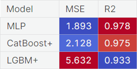
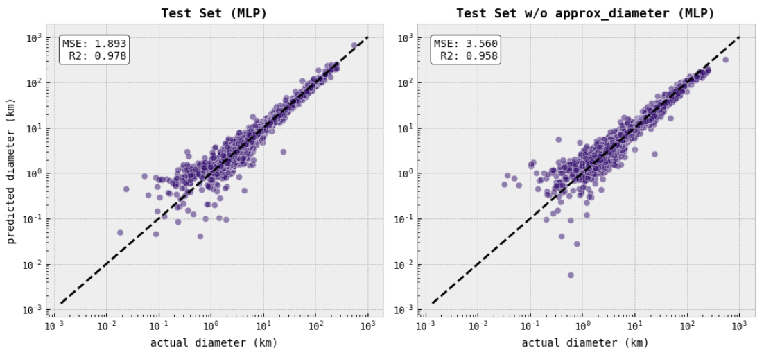
• Identified the MLP model as the top-performing model, achieving an MSE of 1.893 and an R2 score of 0.978 on the test set, surpassing other models.
• Revealed crucial patterns and correlations in a highly imbalanced dataset of 137,000 asteroid observations, providing valuable insights for understanding asteroid behavior, informing the assessment of the potential impact of asteroids on Earth, and planning future space missions to study these objects,
• Discovered critical dataset characteristics, including a dominant class comprising 92% of asteroids, and identified 7% of asteroids with poorly determined orbits, enabling strategic decision-making for accurate and reliable predictions.
• Improved data quality by identifying outliers and missing values in data, which were then processed using appropriate methods such as imputation and removal.
• Constructed robust models for accurate asteroid diameter prediction, crucial for identifying potentially hazardous asteroids and enhancing classification models for distinguishing between hazardous and non-hazardous asteroids.

RESULTS

The project aimed to assess the performance of three models for predicting asteroid diameters: MLP, CatBoost, and LGBM. The evaluation was based on two metrics: mean squared error (MSE) and R2 score.

The MLP model proved to be the most suitable and accurate model for predicting asteroid diameters in this project. Although the MLP model showed the best performance, all three models achieved satisfactory results in predicting asteroid diameters, with the MLP model being the most accurate among them, having achieved an MSE of 1.893 and the highest R2 score of 0.978.

The MSE scores for all models ranged from approximately 1.893 to 5.632, indicating that the average deviation of the predicted diameters from the actual diameters was within a range from 1.375 to 2.373 kilometers for distinct models. The R2 scores, on the other hand, ranged from 0.933 to 0.978, indicating the percentage of the variance in the target variable (diameters) that was explained by the models.

Table of Contents

1. Project At A Glance
2. Introduction
3. Problem Statement and Motivation
4. EDA
5. Feature Engineering and Data Preprocessing
6. Building and Fine-Tuning the Models

Project At A Glance

Python Version: 3.7.12

Packages: numpy, pandas, matplotlib, seaborn, sklearn, tensorflow, lightgbm, catboost.

Introduction

Asteroids are small, rocky objects that revolve around the Sun in elliptical orbits. They are sometimes called minor planets or planetoids and are remnants left over from the early formation of our solar system about 4.6 billion years ago.

Asteroids range in size from tiny specks to hundreds of kilometers across, and they are located primarily in the asteroid belt between Mars and Jupiter, though, they can also be observed in other regions of the solar system. Most asteroids are irregularly shaped, only some of them are close to spherical, and they are often pitted or cratered. But wait, what do we mean by the diameter of the asteroid if it is of irregular shape?

Basically, the diameter of an asteroid of irregular shape is usually represented by its equivalent diameter, which is the diameter of a sphere that has the same volume as the asteroid. This equivalent diameter is a handy way to compare the size of different asteroids, but it should be noted that it does not necessarily represent the actual physical size or shape of the asteroid. In some cases, the equivalent diameter may be an overestimate or an underestimate of the true size of the asteroid, depending on its shape and density.

There are two classes of asteroids that are of particular interest to astronomers and planetary scientists: NEAs and PHAs. NEAs stands for "Near-Earth Asteroids", and, as the name suggests, these are asteroids that come relatively close to Earth's orbit, meaning they have the potential to collide with Earth. On the other hand, PHA stands for "Potentially Hazardous Asteroids" and these are a subset of NEAs that are particularly worrisome because they have the potential to come even closer to Earth's orbit, and their size is big enough that they could cause significant damage if they were to collide with Earth.

Apart from other reasons, diameter prediction is extremely important for identifying NEAs and PHAs, since the size of an asteroid can have a big impact on how it interacts with Earth. Smaller asteroids are more likely to burn up in Earth's atmosphere before reaching the surface, while larger asteroids can cause more damage upon impact. By predicting the diameter of NEAs and PHAs, scientists can better assess the potential threat these asteroids pose to Earth and develop strategies to diminish any potential harm. In addition, the diameter prediction can also provide valuable information about the composition, structure, and evolution of asteroids, which can lead to a deeper understanding of the origins of the Solar System we live in.

Problem Statement and Motivation

This project aims to estimate the size of asteroids in our solar system based on various observable characteristics such as their absolute magnitude, albedo, distance from the Sun, and their orbital parameters. Accurately predicting the size of asteroids is crucial for understanding their potential impact on Earth and for planning future space missions to study these objects.

The project involves analyzing the set of observational data published by JPL’s Solar System Dynamics (SSD) group, to create models that can predict the diameter of asteroids based on their observable characteristics. Ultimately, the goal of the project is to improve our understanding of the asteroid population and its potential impact on our planet.

As someone who is truly fascinated by astronomy and data mining, I am looking forward to working on the project that will help me learn captivating facts about the field I take interest in, not only from the textbook, but from the real astronomical data, and also enhance my skills both through careful attention to the details of data and machine learning, when it comes down to the actual use of the knowledge gained during the analysis.

The outline of the project looks like this:

To begin with, I will be exploring the dataset in search of interesting relationships between the features and explaining the relationships if possible. That is what I will be doing in the Exploring the Data section. Then I will be preparing the data for training the diameter prediction models further in the project. This step comprises feature engineering, encoding the categorical features, and scaling the data. After having done that, the primary focus will be on constructing and fine-tuning three models: MLP neural network, CatBoost, and Light GBM. By exploring and optimizing these models, I aim to identify the most suitable one for our specific task - the prediction of asteroid diameter. Through a comparative analysis of their performance, you will see me make an informed decision about which model yields the best results.

EDA

Please note that if one is willing to see more of the takeaways from the EDA, then I suggest reading the whole notebook, which can be found either on Github or Kaggle.

Here I present some of the highlights from the EDA.

Asteroid Classes, NEAs, PHAs

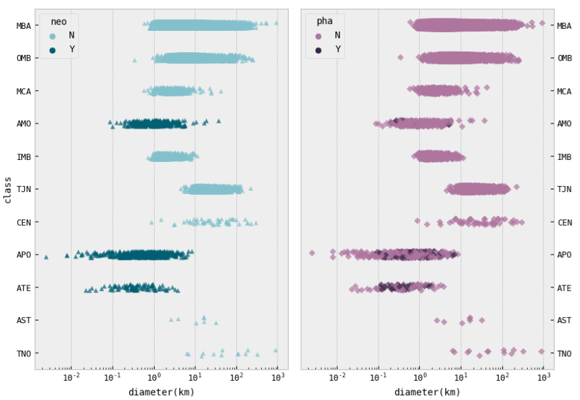
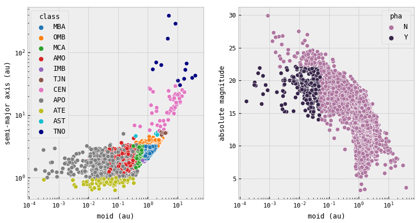
• In the first figure on the right, we see that most of the objects which are considered potentially hazardous are only NEAs of classes AMO, APO, and ATE, these are the asteroids that either cross the Earth's orbit or move close to it in their orbits. We see that most of these asteroids have very low diameters, from 0.1 km to 1 km, with a median of 0.56 km for AMO, 0.59 km for APO, and 0.32 km for ATE.
• From other plots not shown here we also know that there are many more non-dangerous asteroids than those that may be threatening, and even though there are 850 NEAs, only a small fraction of them is considered potentially hazardous.

Condition Code

• The condition code ranges from 0 to 9. The condition code of 0 or 1 indicates a well-determined orbit, while codes 2-4 indicate a less certain orbit, and codes 5-9 indicate a poorly determined orbit.
• In the lower plot on the right, we see that, fortunately, we have a lot of well-determined orbits from almost every class, but we also have a couple of thousands of asteroids with poorly determined orbits, and these are mainly MBAs, OMBs, and IMBs. Since TNOs and CENs orbits are usually large, making it difficult to determine them correctly and also decreasing the opportunities to observe these asteroids, it makes sense that some TNOs and CENs have less certain orbits.
• Some classes of asteroids, such as NEAs, may be of particular interest to researchers and, therefore, may have more observational data and a lower condition code due to the efforts of astronomers to accurately determine their orbits, as we see for ATEs, AMOs, and APOs. However, there are still some of NEAs, such as APOs and AMOs with uncertain orbits. The possible reason for that is that they have really small diameters and may be really difficult to observe, not to mention their short orbital periods.
• Overall, there is no specific relationship between the class and condition code, condition code is rather dependent on the number of observations, and one finds the exploration of this feature in the notebook.

Inclination & Eccentricity

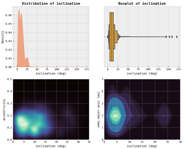
• The upper plot on the right shows that most eccentricities range from 0 deg to 25 deg. We notice that the majority of asteroids have either eccentricities from 0.05 to 0.2 and inclinations from around 2 deg to 7 deg or eccentricities lower than 0.15 and inclinations somewhere around 10 deg. This may be a hint telling us that most of the asteroids in our dataset are MBAs (low eccentricity due to stable orbit). Not to mention that for these values of inclination, we have the range for the semi-major axis from 0.5 au to 3.5 au. Such semi-major axes commonly have MBAs, OMBs, IMBs, APOs, MCAs, AMOs, and ATEs.
• Therefore, the relationship between an asteroid's inclination and eccentricity can provide important information about the class asteroid belongs to and so its overall characteristics.

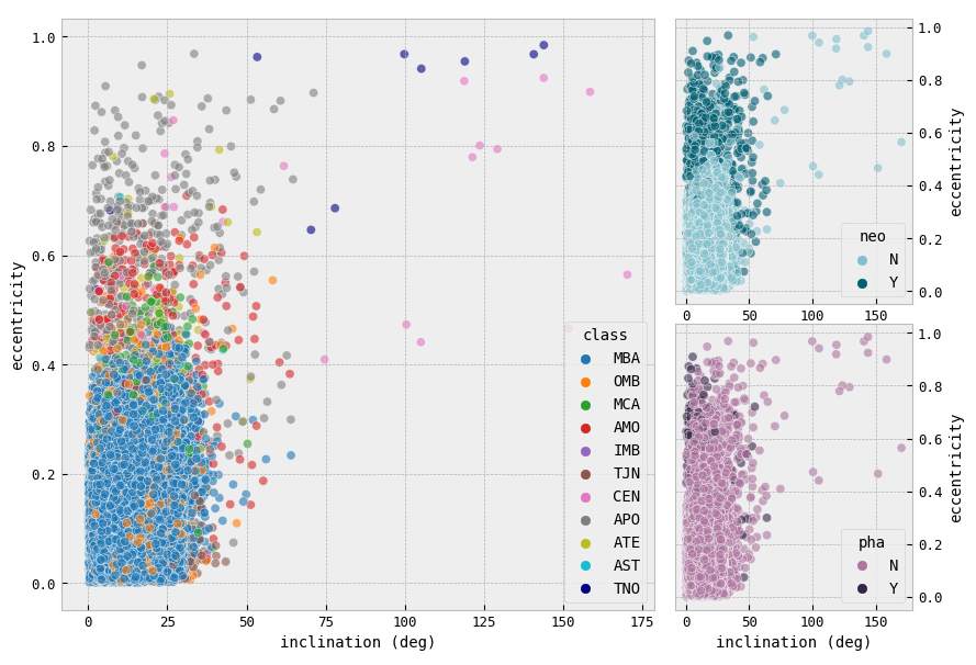
From the lower plots on the right, this can be concluded:

• MBAs typically have low eccentricities and inclinations, which means their orbits are relatively stable.
• MCAs usually have low-inclination but high-eccentricity orbits because they may have been perturbed by the gravity of Mars.
• NEAs have orbits that bring them close to or cross the orbit of Earth. As a result, they tend to have higher eccentricities and inclinations than MBAs. Certain types of NEAs, such as ATEs tend to have higher inclinations than others.
• TJNs are located in stable regions around the Lagrange points of Jupiter's orbit, and they typically have low eccentricities and inclinations.
• CENs are objects that orbit the Sun between Jupiter and Neptune, and they typically have high inclinations and eccentricities since many CENs are believed to have originated in the Kuiper Belt. It suggests that they may have been gravitationally scattered by Neptune or other large planets.
• TNOs have a wide range of eccentricities and inclinations. Some TNOs have highly elliptical and inclined orbits for the same reasons as CENs have too.

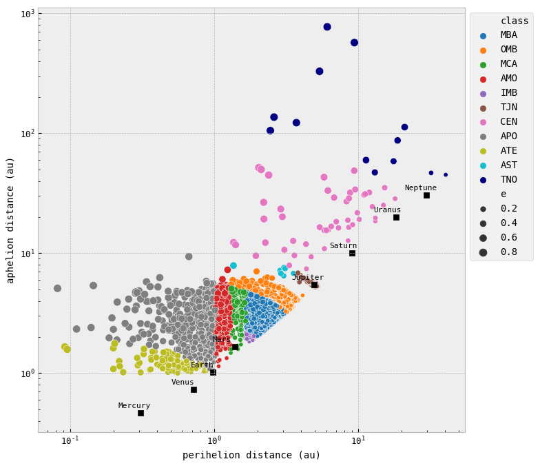
Perihelion & Aphelion distances

• The relationship between aphelion distance and perihelion distance for asteroids of different classes can vary. However, in general, the greater the eccentricity of an asteroid's orbit, the larger the difference between its aphelion and perihelion distances.
• NEAs: all have highly eccentric orbits, which means that their aphelion distance and perihelion distance can differ significantly. ATEs have orbits entirely inside the Earth's orbit but are still close to it, and typically have aphelion distances that are not significantly larger than their perihelion distances. For APOs, which have orbits that are mostly inside the Earth's orbit and cross it, the aphelion distance is typically much larger than the perihelion distance. For AMOs, which have orbits that cross Earth's orbit from the outside, the aphelion distance can be significantly larger than the perihelion distance as well.
• IMBs and OMBs have orbits that are less eccentric than those of NEAs and TNOs. Therefore, their aphelion distance and perihelion distance are typically more similar in value.
• MBAs: Their orbits are mostly circular, with eccentricities typically less than 0.3. This means that their aphelion and perihelion distances are relatively close, therefore, their orbits should be relatively stable and predictable.
• MCAs have orbits that cross the orbit of Mars, which means that their perihelion distances are closer to the Sun than those of IMBs and OMBs. Their aphelion distances can be significantly larger than their perihelion distances, depending on the specific orbit of the asteroid.
• TJNs have orbits that are stabilized by the gravity of Jupiter, which means that their orbits are relatively stable and not highly eccentric. Therefore, their aphelion and perihelion distances are typically not very different from each other.
• CENs and TNOs: They have highly elliptical orbits with eccentricities greater than 0.3. This leads to them having large differences between aphelion and perihelion distances. Their orbits are rather chaotic and hard to predict due to that.

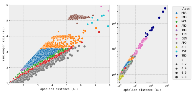
Aphelion distance & Semi-major Axis

• Since the semi-major axis of an asteroid is the average distance between the asteroid and the sun, it determines the overall shape and size of the asteroid's elliptical orbit. The aphelion distance is the point at which the asteroid is farthest from the sun in its orbit, and this distance is directly related to the semi-major axis of the ellipse. Specifically, the aphelion distance is equal to $a(1+e)$.
• In summary, the aphelion distance of an asteroid is related to its semi-major axis through Kepler's laws of planetary motion, specifically through the shape and size of the asteroid's elliptical orbit. The upper plots on the right actually confirm this.

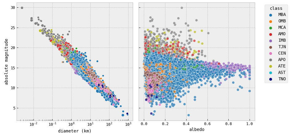
Absolute Magnitude & Albedo

• In general, smaller asteroids have higher absolute magnitudes (i.e., are darker), while larger asteroids have lower absolute magnitudes (i.e., are brighter). Albedo also plays a role, as objects with higher albedo (i.e., they reflect more light) have lower absolute magnitudes.
• If we look at two lower plots, we would conclude that MBAs have a relatively uniform distribution of absolute magnitudes, with a mean value of around $H=13$. There also can be noticed a slight trend for smaller asteroids to have higher absolute magnitudes, and for larger asteroids to have lower absolute magnitudes. This class spans all albedo values. Most of the time asteroids with albedo around 14 may have high albedos (greater than 0.6), but MBAs with $H > 14$ and $H < 14$ usually have $albedo < 0.6$. And the brighter the MBA is, the larger it is, then its albedo gets lower.
• IMBs are known for having high albedos compared to other asteroid classes. This is because they are composed of silicate rocks, which are more reflective than other materials, such as carbonaceous chondrites that are found in outer main belt asteroids. Additionally, many IMBs have undergone space weathering, a process that can make their surfaces brighter by removing the darker outer layer of material and revealing the brighter interior.
• OMBs and MCAs usually have low albedos and follow the general rule of lower H leading to greater size.
• NEAs seem to have higher albedos when they are brighter (absolute magnitude is lower) and larger. Still, despite their proximity to the Sun, their albedos are much lower than these of MBAs sometimes and never are higher than 0.6.
• For TJNs, there is a correlation between absolute magnitude and diameter, with brighter asteroids generally being larger and also having higher albedos.
• The general rule applies to CENs too, since brighter CENs are often larger too, but they do not necessarily have an increase in albedo. Most of them have really low albedos. They have a relatively uniform distribution of absolute magnitudes, with a mean value of around $H=10$.
• TNOs have a wide range of absolute magnitudes. Brighter TNOs generally are larger too, but not less absorptive.

Minimum Orbit Intersection Distance (MOID)

• NEAs are more likely to have smaller MOIDs due to their proximity to Earth and their orbits that intersect Earth's orbit.
• MBAs generally have larger MOIDs because they have more circular orbits and are located farther from Earth.
• Only NEAs whose $moid < 0.05$ and whose $H <= 22.0$ may usually be considered PHAs. And our plot on the right tells us that asteroids in our dataset are entirely in accord with the statement.

Bivariate Distributions

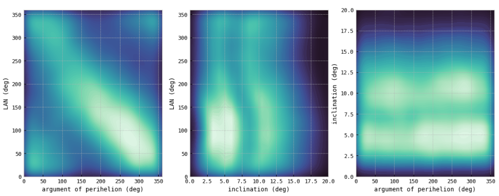
• The last figure shows the probability of two given variables occurring. For example, we see that most of the asteroids have inclinations below 15. deg and these occurrences spread over all values of LAN and argument of perihelion.

Feature Engineering and Data Preprocessing

During the feature engineering and data preprocessing phase, I employed several techniques to optimize the dataset for modeling and analysis. Firstly, I performed feature engineering by creating a new feature called approx_diameter based on existing features. The introduction of the new feature, approx_diameter, played a crucial role in improving the performance of the MLP model. This feature was engineered to capture an approximate diameter value for each asteroid, providing additional information that was not explicitly available in the original dataset.

By incorporating this new feature, the MLP model was able to leverage the relationship between the existing features and the target variable more effectively. The approx_diameter feature likely captured some hidden patterns or correlations that were not apparent in the other features alone. As a result, the MLP model, which is known for its ability to learn complex relationships in data, was able to exploit the information provided by the approx_diameter feature, leading to improved predictions and higher accuracy. The inclusion of this feature might have introduced new insights and nuances into the modeling process, allowing the MLP model to outperform the other models.

This emphasized that by carefully engineering relevant and informative features, we can enhance the performance of our models and uncover hidden patterns in the data. In this case, the approx_diameter feature proved to be a valuable addition, contributing to the success of the MLP model as the best-performing model in the project.

Next, I tackled the categorical features in the dataset by applying one-hot encoding. This technique transformed categorical variables into a binary format, allowing the models to process them effectively. The resulting encoded features provided valuable information for predicting the target variable.

To ensure a fair evaluation of the models' performance, I split the dataset into training, validation, and test sets. The training set was used to train the models, the validation set helped in hyperparameter tuning and model selection, and the test set provided an independent evaluation of the final models' performance.

Furthermore, I applied data scaling techniques, specifically standardization, to normalize the numerical features. This step ensured that all features were on a similar scale, preventing any particular feature from dominating the model's learning process.

Through meticulous feature engineering, proper encoding of categorical features, careful data splitting, and appropriate data scaling, I aimed to create a dataset that was well-suited for modeling and analysis. These steps were crucial in optimizing the data and ensuring that the models could effectively learn patterns and make accurate predictions.

Building and Fine-Tuning the Models

In this section, I trained and compared three different models: MLP, CatBoost, and LightGBM. The models were trained on both the entire dataset and a reduced dataset without the approx_diameter feature and further fine-tuned to improve their performance using the validation set. The performance of the models was evaluated using metrics such as MSE and R2 score.

Initially, training the models on the entire dataset showed that the CatBoost model with the approx_diameter feature performed slightly better, while the MLP model also demonstrated competitive performance. Surprisingly, when training the models on the reduced dataset without the approx_diameter feature, the CatBoost model still performed well and achieved comparable results to the models trained on the entire dataset and was better than any other result so far. This suggests that the CatBoost model was able to capture the important patterns and relationships within the dataset, with or without the engineered feature.

To further optimize the models, I conducted fine-tuning, adjusting the hyperparameters to improve their performance. The fine-tuned models, particularly the LightGBM model, exhibited improved results with reduced MSE and higher R2 scores, indicating enhanced accuracy and predictive power.

To sum up, the comparison of the models highlighted the effectiveness of feature engineering and fine-tuning in improving model performance. The MLP model showcased the importance of the approx_diameter feature, which significantly enhanced its predictions on the test set. Meanwhile, the CatBoost and LightGBM models performed well on both the entire and reduced validation datasets, demonstrating their robustness and ability to capture patterns in unseen data. Despite CatBoost leading on the validation set, the MLP model emerged as the top-performing model on the test set, demonstrating its superior predictive power.