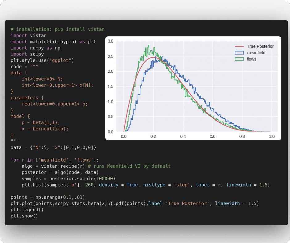
vistan is a simple library to run variational inference algorithms on Stan models.
vistan uses autograd and PyStan under the hood. The aim is to provide a "petting zoo" to make it easy to play around with the different variational methods discussed in the NeurIPS 2020 paper Advances in BBVI.
- Initialization: Laplace's method to initialize full-rank Gaussian
- Gradient Estimators: Total-gradient, STL, DReG, closed-form entropy
- Variational Families: Full-rank Gaussian, Diagonal Gaussian, RealNVP
- Objectives: ELBO, IW-ELBO
- IW-sampling: Posterior samples using importance weighting
pip install vistan
The typical usage of the package would have the following steps:
- Create an algorithm. This can be done in two wasy:
- The easiest is to use a pre-baked recipe as
algo=vistan.recipe('meanfield'). There are various options:'advi': Run our implementation of ADVI's PyStan.'meanfield': Full-factorized Gaussia a.k.a meanfield VI'fullrank': Use a full-rank Gaussian for better dependence between latent variables'flows': Use a RealNVP flow-based VI'method x': Use methods from the paper Advances in BBVI where x is one of[0, 1, 2, 3a, 3b, 4a, 4b, 4c, 4d]
- Alternatively, you can create a custom algorithm as
algo=vistan.algorithm(). Some most frequent arguments:vi_family: This can be one of['gaussian', 'diagonal', 'rnvp'](Default:gaussian)max_iter: The maximum number of optimization iterations. (Default: 100)optimizer: This can be'adam'or'advi'. (Default:'adam')grad_estimator: What gradient estimator to use. Can be'Total-gradient','STL','DReG', or'closed-form-entropy'. (Default:'DReG')M_iw_train: The number of importance samples. Use1for standard variational inference or more for importance-weighted variational inference. (Default: 1)per_iter_sample_budget: The total number of evaluations to use in each iteration. (Default: 100)
- Get an approximate posterior as
posterior=algo(code, data). This runs the algorithm on Stan model given by the stringcodewith observations given by thedata. - Draw samples from the approximate posterior as
samples=posterior.sample(100). You can also draw samples using importance weighting asposterior.sample(100, M_iw_sample=10). Further, you can evaluate the log-probability of the posterior asposterior.log_prob(latents).
If you use vistan, please, consider citing:
@inproceedings{aagrawal2020,
  author    = {Abhinav Agrawal and
               Daniel R. Sheldon and
               Justin Domke},
  title     = {Advances in Black-Box {VI:} Normalizing Flows, Importance Weighting,
               and Optimization},
  booktitle = {Advances in Neural Information Processing Systems 33: Annual Conference
               on Neural Information Processing Systems 2020, NeurIPS 2020, December
               6-12, 2020, virtual},
  year      = {2020},
}
Recipies refers to set of predetermined hyperparameters that let you quickly run some common variational algorithms.
'meanfield' runs the fully factorized Gaussian VI optimized using Adam
import vistan
import matplotlib.pyplot as plt
import numpy as np
import scipy
code = """
data {
    int<lower=0> N;
    int<lower=0,upper=1> x[N];
}
parameters {
    real<lower=0,upper=1> p;
}
model {
    p ~ beta(1,1);
    x ~ bernoulli(p);
}
"""
data = {"N":5, "x":[0,1,0,0,0]}
algo = vistan.recipe() # runs Meanfield VI by default
posterior = algo(code, data)
samples = posterior.sample(100000)

points = np.arange(0,1,.01)
plt.hist(samples['p'], 200, density = True, histtype = 'step')
plt.plot(points,scipy.stats.beta(2,5).pdf(points),label='True Posterior')
plt.legend()
plt.show()'fullrank', as the name suggests, optimizes full-rank Gaussian VI using Adam
algo = vistan.recipe("fullrank")
posterior = algo(code, data)
samples = posterior.sample(100000)

points = np.arange(0, 1, .01)
plt.hist(samples['p'], 200, density=True, histtype='step')
plt.plot(points, scipy.stats.beta(2, 5).pdf(points), label='True Posterior')
plt.legend()
plt.show()'flows' optimizes a RealNVP inspired flow distribution for variational approximation using Adam
algo = vistan.recipe("flows")
posterior = algo(code, data)
samples = posterior.sample(100000)

points = np.arange(0, 1, .01)
plt.hist(samples['p'], 200, density=True, histtype='step')
plt.plot(points, scipy.stats.beta(2, 5).pdf(points), label='True Posterior')
plt.legend()
plt.show()'advi' runs our implementation of PyStan's ADVI and uses their custom step-sequence scheme
algo = vistan.recipe("advi")
posterior = algo(code, data)
samples = posterior.sample(100000)

points = np.arange(0, 1, .01)
plt.hist(samples['p'], 200, density=True, histtype='step')
plt.plot(points, scipy.stats.beta(2, 5).pdf(points), label='True Posterior')
plt.legend()
plt.show()
Methods from Advances in BBVI
method x runs implementation of different variational methods from Advances in BBVI, where x is one of [0, 1, 2, 3a, 3b, 4a, 4b, 4c, 4d]
# Try method 0, 1, 2, 3a, 3b, 4a, 4b, 4c, 4d
algo = vistan.recipe("method 4d")
posterior = algo(code, data)
samples = posterior.sample(100000)

points = np.arange(0, 1, .01)
plt.hist(samples['p'], 200, density=True, histtype='step')
plt.plot(points, scipy.stats.beta(2, 5).pdf(points), label='True Posterior')
plt.legend()
plt.show()You can also specify custom VI algorithms to work with your Stan models using vistan.algorithm. Please, see the documentation of vistan.algorithm for a complete list of supported arguments.
algo = vistan.algorithm(
                M_iw_train=2,
                grad_estimator="DReG",
                vi_family="gaussian",
                per_iter_sample_budget=10,
                max_iters=100)
posterior = algo(code, data)
samples = posterior.sample(100000)

points = np.arange(0, 1, .01)
plt.hist(samples['p'], 200, density=True, histtype='step')
plt.plot(points, scipy.stats.beta(2, 5).pdf(points), label='True Posterior')
plt.legend()
plt.show()We provide support to use IW-sampling at inference time; this importance weights M_iw_sample candidate samples and picks one (see Advances in BBVI for more information.) IW-sampling is a post-hoc step and can be used with almost any variational scheme.
samples = posterior.sample(100000, M_iw_sample=10)

points = np.arange(0, 1, .01)
plt.hist(samples['p'], 200, density=True, histtype='step')
plt.plot(points, scipy.stats.beta(2, 5).pdf(points), label='True Posterior')
plt.legend()
plt.show()We provide support to use Laplace's method to initialize the parameters for Gaussian VI.
algo = vistan.algorithm(vi_family='gaussian', LI=True)
posterior = algo(code, data)
samples = posterior.sample(100000)

points = np.arange(0, 1, .01)
plt.hist(samples['p'], 200, density=True, histtype='step')
plt.plot(points, scipy.stats.beta(2, 5).pdf(points), label='True Posterior')
plt.legend()
plt.show()We provide access to the model.log_prob function we use internally for optimization. This allows you to evaluate the log density in the unconstrained space for your Stan model. Also, this function is differentiable in autograd.
log_prob = posterior.model.log_prob
- We currently only support inference on all latent parameters in the model
- No support for data sub-sampling.
