This solution assumes that you have already executed this notebook up to the bottom, so that all data is already loaded.
First, remember that we had a nodata value of -9999 for the population layer. Let's replace that with 0 first to get the proper population numbers:
pop[pop < 0] = 0
(In fact, that is a quick and dirty fix. You can read more about handling nodata masks in Rasterio in the documentation.)
Then we'll select all urban cells:
u = urban == 2... and then loop over the country IDs, and for each country:
- Select cells that are within that country from the population raster and add them up;
- Select cells that are within that country and urban using np.all from the population raster and add them up:
for c in np.unique(countries):

    incountry = countries == c

    print(c, "total:", "{:,}".format(np.sum(pop[incountry])))
    print(c, "urban:", "{:,}".format(np.sum(pop[np.all((incountry, u), axis=0)])))
Output:
0 total: 0
0 urban: 0
12 total: 38,615,393
12 urban: 23,453,970
24 total: 22,163,601
24 urban: 11,015,239
72 total: 2,422,366
72 urban: 1,226,879
108 total: 8,381,284
108 urban: 920,779
120 total: 22,517,640
120 urban: 11,312,845
132 total: 499,673
132 urban: 279,265
140 total: 4,532,869
140 urban: 1,701,565
148 total: 11,650,688
148 urban: 3,101,414
...
Generate a raster that indicates the distance to the closest urban cell for every cell in the output raster and visualize that raster
For the cost distance, we need to know the indexes of the urban cells. np.where does that:
u = np.where(urban == 2)
u
As you can see, this gives us a tuple with the coordinates for each cell where the urban layer has a value of 2:
(array([   1,    1,    1, ..., 8633, 8633, 8633]),
 array([4220, 4221, 4222, ..., 5364, 5365, 5371]))
The first array holds the x indexes, the second one the y indexes. Unfortunately, we need a list of pairs for the find_costs function. Luckily, zip does exactly that:
urbanIndexes = [(x,y) for x,y in zip(u[0], u[1])]
urbanIndexes
Zip allows us to walk through both arrays at the same time. We use that here to take the first element from array 1 and combine it with the first element of the array 2, then the second from array 1 with the second from array 2, and so on.
Output:
[(1, 4220),
 (1, 4221),
 (1, 4222),
 (1, 4223),
 (2, 4219),
 (2, 4220),
 (2, 4221),
 (2, 4222),
 (2, 4223),
 (2, 4224),
 (2, 4225),
 ...
So those are the source locations for our cost distance. Now we need the actual costs – in our previous example, we took elevation. Since we only care about distance here, we will just assign each cell the value one, using np.ones_like:
fake_cost = np.ones_like(pop)
fake_cost
Output:
array([[1, 1, 1, ..., 1, 1, 1],
       [1, 1, 1, ..., 1, 1, 1],
       [1, 1, 1, ..., 1, 1, 1],
       ...,
       [1, 1, 1, ..., 1, 1, 1],
       [1, 1, 1, ..., 1, 1, 1],
       [1, 1, 1, ..., 1, 1, 1]], dtype=int16)
(Note that we make the simplifying assumption here that all cells have the same size, which is not the case, as we discussed yesterday! If we wanted to do that properly, we would need to reproject all of the Africa data to an equal area projection first. Then we could use the actual cell size to give us a realistic distance to the closest urban cell.)
With all the preparation done, we can now calculate the cost surface (this takes a while for all of Africa...):
lg = graph.MCP_Geometric(fake_cost)
lcd = lg.find_costs(starts=urbanIndexes)[0]
... and plot it:
plt.figure(figsize=(14, 14))
imgplot = plt.imshow(lcd, norm=LogNorm(), cmap='hot')
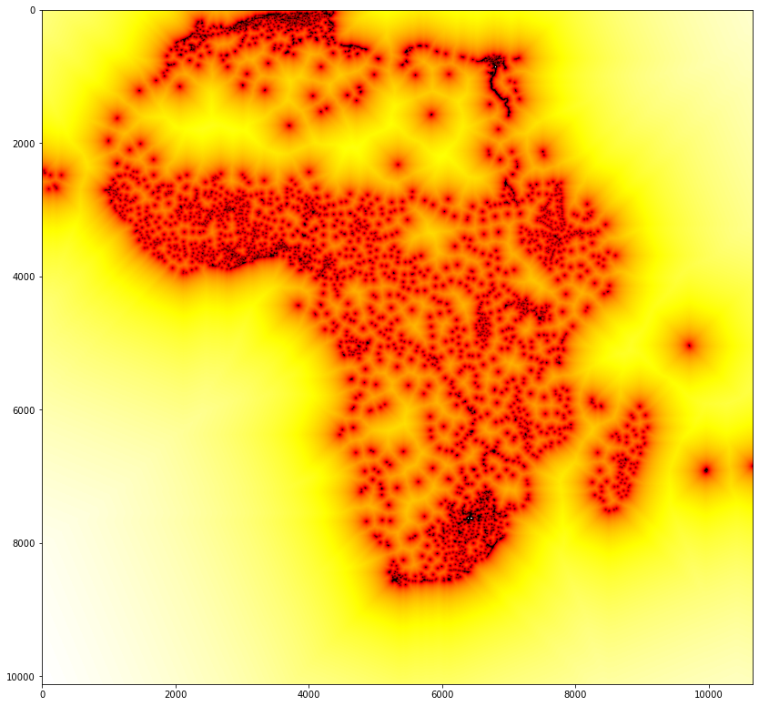
¯\_(ツ)_/¯