Green's function

Green's function of an atomic chain

This example demonstrates a computation of the retarded Green's function function of an atomic chain. The chain consists of identical atoms of an abstract chemical element, say an element "A".

    import sys
    import numpy as np
    import matplotlib.pyplot as plt
    import tb
    import negf
    
    xyz_file = """1
    H cell
    A1       0.0000000000    0.0000000000    0.0000000000                                                                                                      
    """
    
    a = tb.Orbitals('A')

 _   _                   _   _      _   
| \ | | __ _ _ __   ___ | \ | | ___| |_ 
|  \| |/ _` | '_ \ / _ \|  \| |/ _ \ __|
| |\  | (_| | | | | (_) | |\  |  __/ |_ 
|_| \_|\__,_|_| |_|\___/|_| \_|\___|\__|

Let us assume each atomic site has one s-type orbital and the energy level of -0.7 eV. The coupling matrix element equals -0.5 eV.

    a.add_orbital('s', -0.7)
    tb.Orbitals.orbital_sets = {'A': a}
    tb.set_tb_params(PARAMS_A_A={'ss_sigma': -0.5})

With all these parameters we can create an instance of the class Hamiltonian. The distance between nearest neighbours is set to 1.1 A.

    h = tb.Hamiltonian(xyz=xyz_file, nn_distance=1.1).initialize()

The verbosity level is 2
The radius of the neighbourhood is 1.1 Ang

---------------------------------

The xyz-file:
 1
H cell
A1       0.0000000000    0.0000000000    0.0000000000                                                                                                      

---------------------------------

Basis set 
 Num of species {'A': 1} 


 A 
title | energy | n | l | m | s
------+--------+---+---+---+--
s     | -0.7   | 0 | 0 | 0 | 0
------+--------+---+---+---+--
 
---------------------------------

Radial dependence function: None

---------------------------------

Discrete radial dependence function: None

---------------------------------

Unique distances: 
    
---------------------------------

Now we need to set periodic boundary conditions with a one-dimensional unit cell and lattice constant of 1 A.

    h.set_periodic_bc([[0, 0, 1.0]])

Primitive_cell_vectors: 
 [[0, 0, 1.0]] 

---------------------------------

    h_l, h_0, h_r = h.get_hamiltonians()

    energy = np.linspace(-3.5, 2.0, 500)

    sgf_l = []
    sgf_r = []

    for E in energy:
        L, R = negf.surface_greens_function(E, h_l, h_0, h_r)
        sgf_l.append(L)
        sgf_r.append(R)

    sgf_l = np.array(sgf_l)
    sgf_r = np.array(sgf_r)

    num_sites = h_0.shape[0]
    gf = np.linalg.pinv(np.multiply.outer(energy+0.001j, np.identity(num_sites)) - h_0 - sgf_l - sgf_r)

    dos = -np.trace(np.imag(gf), axis1=1, axis2=2)

    tr = np.zeros((energy.shape[0]), dtype=np.complex)

    for j, E in enumerate(energy):
        gf0 = np.matrix(gf[j, :, :])
        gamma_l = 1j * (np.matrix(sgf_l[j, :, :]) - np.matrix(sgf_l[j, :, :]).H)
        gamma_r = 1j * (np.matrix(sgf_r[j, :, :]) - np.matrix(sgf_r[j, :, :]).H)
        tr[j] = np.real(np.trace(gamma_l * gf0 * gamma_r * gf0.H))
        dos[j] = np.real(np.trace(1j * (gf0 - gf0.H)))
   

/home/mk/TB_project/tb_env3/lib/python3.6/site-packages/tb/diatomic_matrix_element.py:115: RuntimeWarning: divide by zero encountered in double_scalars
  prefactor = ((0.5 * (1 + N)) ** l) * (((1 - N) / (1 + N)) ** (m1 * 0.5 - m2 * 0.5)) * \
/home/mk/TB_project/tb_env3/lib/python3.6/site-packages/tb/diatomic_matrix_element.py:123: RuntimeWarning: divide by zero encountered in double_scalars
  ans += ((-1) ** t) * (((1 - N) / (1 + N)) ** t) / \

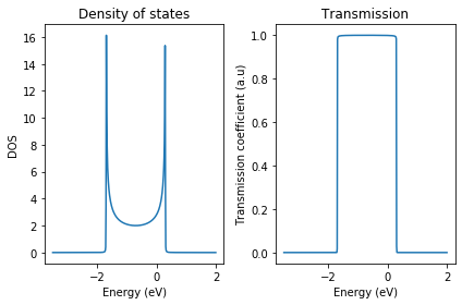
fig, ax = plt.subplots(1, 2)
ax[0].plot(energy, dos)
ax[0].set_xlabel('Energy (eV)')
ax[0].set_ylabel('DOS')
ax[0].set_title('Density of states')

ax[1].plot(energy, tr)
ax[1].set_xlabel('Energy (eV)')
ax[1].set_ylabel('Transmission coefficient (a.u)')
ax[1].set_title('Transmission')
fig.tight_layout()
plt.show()

/home/mk/TB_project/tb_env3/lib/python3.6/site-packages/numpy/core/numeric.py:492: ComplexWarning: Casting complex values to real discards the imaginary part
  return array(a, dtype, copy=False, order=order)

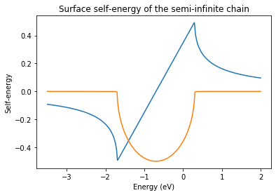
ax = plt.axes()
ax.set_title('Surface self-energy of the semi-infinite chain')
ax.plot(energy, np.real(np.squeeze(sgf_l)))
ax.plot(energy, np.imag(np.squeeze(sgf_l)))
ax.set_xlabel('Energy (eV)')
ax.set_ylabel('Self-energy')
plt.show()