averaging_method

Averaging method

baptiste Auguié -- 22 June, 2014

Three options are provided for angular averaging: Gauss-Legendre quadrature, regular grid in (theta, phi), and a quasi-random Monte Carlo sequence on the sphere. Here we compare their performance and accuracy.

Cluster definitions

gold <- epsAu(seq(600, 800))

cl <- cluster_dimer(d=100, 
              dihedral=10*pi/180, alpha1=20*pi/180, alpha2=0,
              a=35, b=12)

# achiral cluster (plane of symmetry)
cl2 <- cluster_dimer(d=100, 
              dihedral=0*pi/180, alpha1=20*pi/180, alpha2=0,
              a=35, b=12)

Comparison

params <- expand.grid(Nquad=c(10, 50, 100, 1000),
                       averaging=c("grid", "GL", "QMC"),
                       stringsAsFactors=FALSE)

comparison <- mdply(params, circular_dichroism_spectrum, cluster=cl, material=gold)
cheap <- circular_dichroism_spectrum(cluster=cl, material=gold, averaging="cheap")
converged <- circular_dichroism_spectrum(cluster=cl, material=gold, averaging="QMC", Nquad=5000)

p <- 
  ggplot(subset(comparison, type == "CD" & variable == "extinction"),
         aes(wavelength, value)) + 
  facet_grid(averaging~., scales="free")+
  geom_path(aes(colour=factor(Nquad), group=Nquad))+
  geom_path(data=subset(cheap, type == "CD" & variable == "extinction"), linetype=2)+
  geom_path(data=subset(converged, type == "CD" & variable == "extinction"))+
  labs(y=expression(sigma[ext]/nm^2),
       x=expression(wavelength/nm), colour=expression(N))

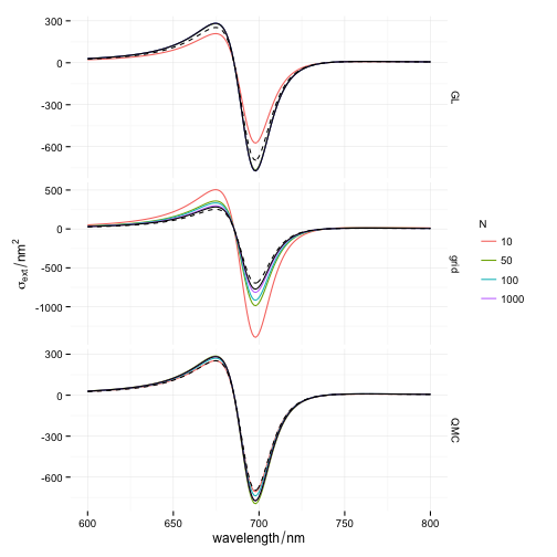
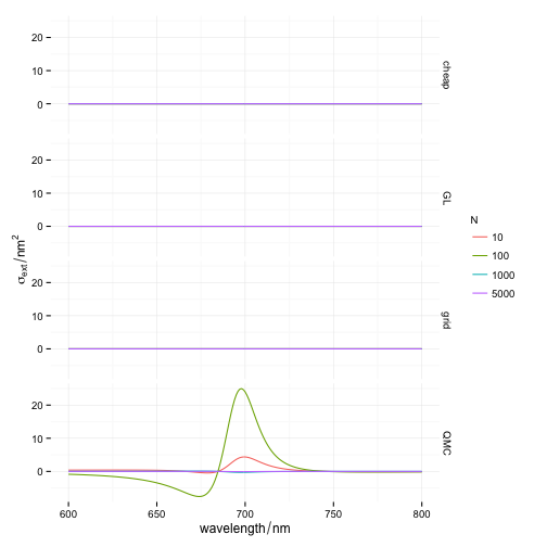
p

The dashed line is a "cheap" version of angular averaging, using only 4 orthogonal directions; it is reasonably close to the converged solution (solid line). QMC seems to perform best in terms of convergence, however, GL may appear more reliable when taking into account symmetry considerations: if a dimer is achiral, the CD signal should be zero. Because QMC uses uneven points on the sphere, it has a harder time at converging towards 0 in such cases.

params <- expand.grid(Nquad=c(10, 100, 1000, 5000),
                       averaging=c("grid", "GL", "QMC", "cheap"),
                       stringsAsFactors=FALSE)

comparison <- mdply(params, circular_dichroism_spectrum, cluster=cl2, material=gold)

p <- 
  ggplot(subset(comparison, type == "CD" & variable == "extinction")) + 
  facet_grid(averaging~.)+
  geom_path(aes(wavelength, value, colour=factor(Nquad), group=Nquad))+
  labs(y=expression(sigma[ext]/nm^2),
       x=expression(wavelength/nm), colour=expression(N))

p