-
Notifications
You must be signed in to change notification settings - Fork 0
/
README.Rmd
137 lines (103 loc) · 4.61 KB
/
README.Rmd
1
2
3
4
5
6
7
8
9
10
11
12
13
14
15
16
17
18
19
20
21
22
23
24
25
26
27
28
29
30
31
32
33
34
35
36
37
38
39
40
41
42
43
44
45
46
47
48
49
50
51
52
53
54
55
56
57
58
59
60
61
62
63
64
65
66
67
68
69
70
71
72
73
74
75
76
77
78
79
80
81
82
83
84
85
86
87
88
89
90
91
92
93
94
95
96
97
98
99
100
101
102
103
104
105
106
107
108
109
110
111
112
113
114
115
116
117
118
119
120
121
122
123
124
125
126
127
128
129
130
131
132
133
134
135
136
137
---
output: github_document
---
```{r, include = FALSE}
knitr::opts_chunk$set(
collapse = TRUE,
comment = "#>",
fig.path = "man/figures/README-",
out.width = "100%"
)
```
# fisheye <img src="man/figures/logo.png" align="right" width="140"/>
<!-- badges: start -->

[](https://app.codecov.io/gh/riatelab/fisheye?branch=main)
[](https://github.com/riatelab/fisheye/actions/workflows/R-CMD-check.yaml)
<!-- badges: end -->
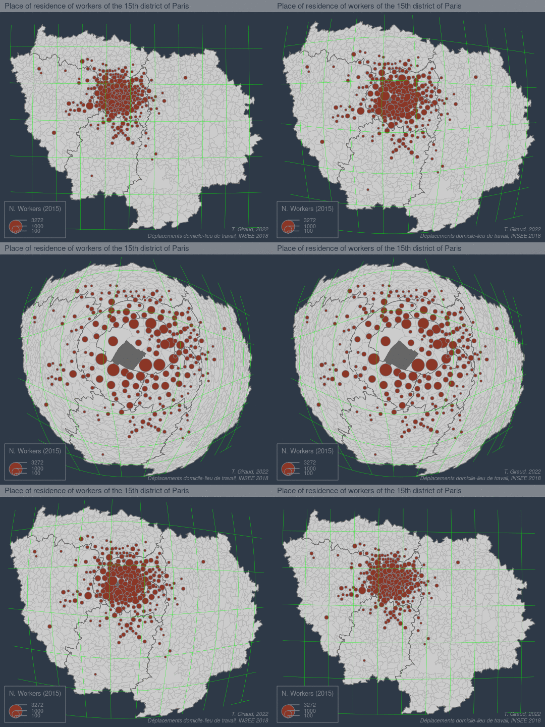
The goal of fisheye is to create base maps focusing on a specific location using an azimuthal logarithmic distance transformation.
<img src="man/figures/fig.jpg" width="350"/>
<small>John Bachmann, [New York and environs](https://digitalcollections.nypl.org/items/510d47e3-b9bd-a3d9-e040-e00a18064a99), 1859.</small>
## Installation
You can install the released version of `fisheye` from
[CRAN](https://cran.r-project.org/package=fisheye) with:
``` r
install.packages("fisheye")
```
Alternatively, you can install the development version of `fisheye` from
GitHub with:
``` r
remotes::install_github("riatelab/fisheye")
```
## Example
This is a basic example:
```{r example, fig.width=10, fig.height = 3, out.width="100%"}
library(sf)
library(fisheye)
library(mapsf)
# Import dataset
ncraw <- st_read(system.file("shape/nc.shp", package="sf"), quiet = TRUE)
nc <- st_transform(ncraw, 3857)
par(mfrow = c(1,2))
mf_map(nc, col ="grey90")
mf_map(nc[51, ], add = TRUE, col = "grey40")
mf_title("Original Map")
# transform the basemap
nc_fe <- fisheye(nc, centre = nc[51, ])
mf_map(nc_fe, col ="grey90")
mf_map(nc_fe[51, ], add = TRUE, col = "grey40")
mf_title("Log-Azimuthal Projection")
```
```{r example2,fig.width=10, fig.height = 3, out.width="100%", echo=FALSE }
# data import
par(mfrow = c(1,2))
mf_theme(mar = c(0.5,0.5,0.5,0.5))
center <- st_centroid(st_geometry(nc[51, ]))
buf_size <- c(
seq(100,1000, 100),
seq(1000,10000,1000),
seq(10000, 100000, 10000)
)
lb <- vector("list", length(buf_size))
for (i in seq_along(lb)){
lb[[i]] <- st_buffer(center, buf_size[i])
}
buf <- st_sf(geom = do.call(c, lb))
mf_init(nc)
mf_map(nc, col ="grey90", border = "white", add = TRUE)
mf_map(buf, add = TRUE, border = "red", col = NA, lwd = .4, lty = 3)
mf_map(buf[c(10,20,30), ], add = TRUE, border = "red", col = NA,
lwd = 1, lty = 1)
mf_map(center, pch = 20, add = TRUE)
for (i in c(20, 30)){
text(x = st_coordinates(center)[1,1],
y = st_bbox(buf[i, ])[4],
labels = paste0(round(buf_size[i]/1000, 0), "km")
)
}
buffe <- fisheye(buf, centre = center, method = "log", k = 1)
ncfe <- fisheye(nc, centre = center, method = "log", k = 1)
mf_init(buffe)
mf_map(ncfe, add = TRUE)
mf_map(buffe, add = TRUE, border = "red", col = NA, lwd = .4, lty = 3)
mf_map(buffe[c(1,10,20,30), ], add = TRUE, border = "red", col = NA,
lwd = 1, lty = 1)
points(0,0,pch = 20)
for (i in c(1,10,20,30)){
text(x = 0,
y = st_bbox(buffe[i, ])[4],
labels = paste0(signif(buf_size[i]/1000, 0), "km")
)
}
```
See a more detailed example [here](https://github.com/rcarto/fisheye-example/):

## References
* Hägerstrand, T. (1957). Migration and Area: A Survey of a Sample of Swedish Migration Fields and Hypothetical Considerations of their Genesis. Lund Studies in Geography, Series B, Human Geography, Department of Geography, University of Lund, Lund.
* Snyder, J.P. (1987). "Magnifying-Glass" Azimuthal Map Projections. The American Cartographer, 14:1, 61-68, https://doi.org/10.1559/152304087783875318
* Fairbairn, D., & Taylor, G. (1995). Developing a variable-scale map projection for urban areas. Computers & Geosciences, 21:9, 1053-1064, https://doi.org/10.1016/0098-3004(95)00041-6
* Boutoura, C., Tsioukas, V., & Tsorlini, A. (2012). Experimenting “fisheye-lens functions” in studying digitally particular historic maps. e-Perimetron (ISSN 1790 - 3769). 7. 111-123. http://www.e-perimetron.org/Vol_7_3/Boutoura_et_al.pdf
* Roughan, M. (2017). Log-azimuthal maps. https://roughan.info/math/log-az/
* Rivière, P. (2018). The Log-Azimuthal projection. https://observablehq.com/@fil/log-azimuthal
* Jansen, T. (2018). “Magnifying-Glass” projections. https://observablehq.com/@toja/magnifying-glass-projections
* Sahasrabuddhe, R., Lambiotte, R., & Alessandretti, L. (2021). From centre to centres: polycentric structures in individual mobility. https://arxiv.org/pdf/2108.08113.pdf