-
Notifications
You must be signed in to change notification settings - Fork 1
/
README.Rmd
226 lines (185 loc) · 6.04 KB
/
README.Rmd
1
2
3
4
5
6
7
8
9
10
11
12
13
14
15
16
17
18
19
20
21
22
23
24
25
26
27
28
29
30
31
32
33
34
35
36
37
38
39
40
41
42
43
44
45
46
47
48
49
50
51
52
53
54
55
56
57
58
59
60
61
62
63
64
65
66
67
68
69
70
71
72
73
74
75
76
77
78
79
80
81
82
83
84
85
86
87
88
89
90
91
92
93
94
95
96
97
98
99
100
101
102
103
104
105
106
107
108
109
110
111
112
113
114
115
116
117
118
119
120
121
122
123
124
125
126
127
128
129
130
131
132
133
134
135
136
137
138
139
140
141
142
143
144
145
146
147
148
149
150
151
152
153
154
155
156
157
158
159
160
161
162
163
164
165
166
167
168
169
170
171
172
173
174
175
176
177
178
179
180
181
182
183
184
185
186
187
188
189
190
191
192
193
194
195
196
197
198
199
200
201
202
203
204
205
206
207
208
209
210
211
212
213
214
215
216
217
218
219
220
221
222
223
224
225
226
---
title: The 'RCDT' package - constrained 2D Delaunay triangulation
output: github_document
editor_options:
chunk_output_type: console
---
<!-- badges: start -->
[](https://github.com/stla/RCDT/actions/workflows/R-CMD-check.yaml)
<!-- badges: end -->

```{r setup, include=FALSE}
knitr::opts_chunk$set(echo = TRUE, collapse = TRUE)
```
## The pentagram
```{r}
# vertices
R <- sqrt((5-sqrt(5))/10) # outer circumradius
r <- sqrt((25-11*sqrt(5))/10) # circumradius of the inner pentagon
X <- R * vapply(0L:4L, function(i) cos(pi/180 * (90+72*i)), numeric(1L))
Y <- R * vapply(0L:4L, function(i) sin(pi/180 * (90+72*i)), numeric(1L))
x <- r * vapply(0L:4L, function(i) cos(pi/180 * (126+72*i)), numeric(1L))
y <- r * vapply(0L:4L, function(i) sin(pi/180 * (126+72*i)), numeric(1L))
vertices <- rbind(
c(X[1L], Y[1L]),
c(x[1L], y[1L]),
c(X[2L], Y[2L]),
c(x[2L], y[2L]),
c(X[3L], Y[3L]),
c(x[3L], y[3L]),
c(X[4L], Y[4L]),
c(x[4L], y[4L]),
c(X[5L], Y[5L]),
c(x[5L], y[5L])
)
```
```{r}
# edge indices (pairs)
edges <- cbind(1L:10L, c(2L:10L, 1L))
```
```{r}
# constrained Delaunay triangulation
library(RCDT)
del <- delaunay(vertices, edges)
```
```{r, eval=FALSE}
# plot
opar <- par(mar = c(0, 0, 0, 0))
plotDelaunay(
del, type = "n", asp = 1, fillcolor = "distinct", lwd_borders = 3,
xlab = NA, ylab = NA, axes = FALSE
)
par(opar)
```
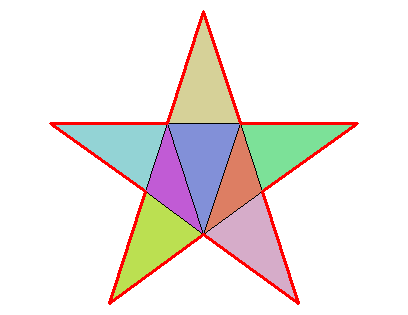
```{r}
# area
delaunayArea(del)
sqrt(650 - 290*sqrt(5)) / 4 # exact value
```
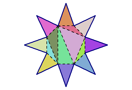
## An eight-pointed star
I found its vertices with the Julia library
[Luxor](http://juliagraphics.github.io/Luxor.jl/v0.10.3/index.html).
```{r}
vertices <- rbind(
c(2.121320343559643, 2.1213203435596424),
c(0.5740251485476348, 1.38581929876693),
c(0.0, 3.0),
c(-0.5740251485476346, 1.38581929876693),
c(-2.1213203435596424, 2.121320343559643),
c(-1.38581929876693, 0.5740251485476349),
c(-3.0, 0.0),
c(-1.3858192987669302, -0.5740251485476345),
c(-2.121320343559643, -2.1213203435596424),
c(-0.5740251485476355, -1.3858192987669298),
c(0.0, -3.0),
c(0.574025148547635, -1.38581929876693),
c(2.121320343559642, -2.121320343559643),
c(1.3858192987669298, -0.5740251485476355),
c(3.0, 0.0),
c(1.38581929876693, 0.5740251485476349)
)
```
```{r}
# edge indices
edges <- cbind(1L:16L, c(2L:16L, 1L))
```
```{r}
library(RCDT)
del <- delaunay(vertices, edges)
```
```{r, eval=FALSE}
opar <- par(mar = c(0, 0, 0, 0))
plotDelaunay(
del, type = "n", asp = 1, fillcolor = "distinct",
col_borders = "navy", lty_edges = 2, lwd_borders = 3, lwd_edges = 2,
xlab = NA, ylab = NA, axes = FALSE
)
par(opar)
```
## Triangulation of a polygon with a hole
```{r polygon_hole}
n <- 100L # outer number of sides
angles1 <- seq(0, 2*pi, length.out = n + 1L)[-1L]
outer_points <- cbind(cos(angles1), sin(angles1))
m <- 10L # inner number of sides
angles2 <- seq(0, 2*pi, length.out = m + 1L)[-1L]
inner_points <- 0.5 * cbind(cos(angles2), sin(angles2))
points <- rbind(outer_points, inner_points)
# constraint edges
indices <- 1L:n
edges_outer <- cbind(
indices, c(indices[-1L], indices[1L])
)
indices <- n + 1L:m
edges_inner <- cbind(
indices, c(indices[-1L], indices[1L])
)
edges <- rbind(edges_outer, edges_inner)
# constrained Delaunay triangulation
del <- delaunay(points, edges)
```
```{r plot_polygon_with_hole, eval=FALSE}
# plot
opar <- par(mar = c(0, 0, 0, 0))
plotDelaunay(
del, type = "n", asp = 1, lwd_borders = 3, col_borders = "black",
fillcolor = "random", col_edges = "yellow",
axes = FALSE, xlab = NA, ylab = NA
)
par(opar)
```
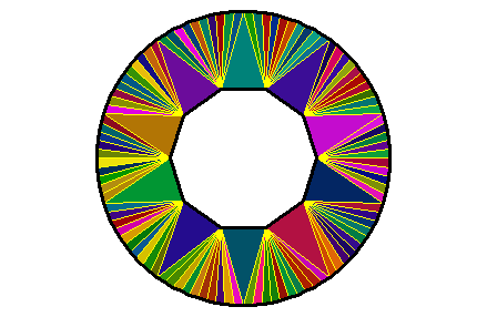
One can also enter a vector of colors in the `fillcolor` argument. First,
see the number of triangles:
```{r number_triangles}
del[["mesh"]]
```
There are 110 triangles. Let's make a cyclic vector of 110 colors:
```{r palette}
colors <- viridisLite::viridis(55)
colors <- c(colors, rev(colors))
```
And let's plot now:
```{r plot_viridis, eval=FALSE}
opar <- par(mar = c(0, 0, 0, 0))
plotDelaunay(
del, type = "n", asp = 1, lwd_borders = 3, col_borders = "black",
fillcolor = colors, col_edges = "black", lwd_edges = 1.5,
axes = FALSE, xlab = NA, ylab = NA
)
par(opar)
```
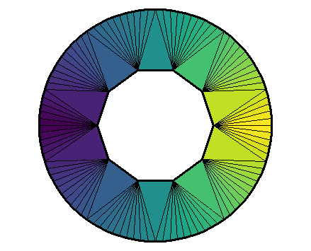
The colors are assigned to the triangles in the order they are given, but only
after the triangles have been circularly ordered.
## A funny curve
I found this curve [here](https://health.ahs.upei.ca/KubiosHRV/MCR/toolbox/matlab/demos/html/demoDelaunayTri.html#19).
```{r suncurve}
t_ <- seq(-pi, pi, length.out = 193L)[-1L]
r_ <- 0.1 + 5*sqrt(cos(6*t_)^2 + 0.7^2)
xy <- cbind(r_*cos(t_), r_*sin(t_))
edges1 <- cbind(1L:192L, c(2L:192L, 1L))
inner <- which(r_ == min(r_))
edges2 <- cbind(inner, c(tail(inner, -1L), inner[1L]))
del <- delaunay(xy, edges = rbind(edges1, edges2))
```
```{r plot_suncurve, eval=FALSE}
opar <- par(mar = c(0, 0, 0, 0))
plotDelaunay(
del, type = "n", col_borders = "black", lwd_borders = 2,
fillcolor = "random", col_edges = "white",
axes = FALSE, xlab = NA, ylab = NA, asp = 1
)
polygon(xy[inner, ], col = "#ffff99")
par(opar)
```

## License
The 'RCDT' package as a whole is distributed under GPL-3 (GNU GENERAL
PUBLIC LICENSE version 3).
It uses the C++ library [CDT](https://github.com/artem-ogre/CDT) which is
permissively licensed under MPL-2.0. A copy of the 'CDT' license is provided in
the file **LICENSE.note**, and the source code of this library can be found in
the **src** folder.