ControlBootcamp_Notes_Mahesh.md

Optimal and Modern Control Theory

Table of Contents:

1. Overview
   1. Objective
   2. Types of Control
2. Linear systems
3. Stability and Eigenvalues
4. Linearizing Around a Fixed Point
5. Controllability
6. Inverted Pendulum on a Cart
7. Pole Placement for the Inverted Pendulum on a Cart
8. LQR Control for the Inverted Pendulum on a Cart
9. Full State Esimation

---

Overview

Objective

1. Writing discription of control system in terms of linear differential equation of inputs and outputs
2. Simulating system
3. Designing controllers to manipulate behavior of system

Types of control

1. Passive: one time solution, no energy expenditure
2. Active: Uses energy
   1. Open loop: Finding optimal constant input for desired output. Example of open loop control.
   2. Closed loop feedback control: using controller to manipulate input depending on current state of system. Uses less energy and more precise. Example of closed loop feedback control

	Open Loop	Closed Loop Feedback control
Uncertainty refers to internal changes in system.	Uncertainty makes input suboptimal.	Uncertainty is not an issue, as any change is system variables gets detected and input is varied accordingly.
	Instable	Very stable.
Disturbance referes to external forces.	Cannot take in account for disturbance.	Disturbance also gets detected by sensors and input is vaired accordingly.
	Inefficient as energy is used continuously	Efficient as energy is used only when required

---

Linear systems

A system can be represented by linear system of differential equation as below.

$$ dx/dt = Ax $$

Here x is a vector consisting system coordinates and A is matrix which represents how these variables interact with each other.

Basic solution of this equation can be given as

$$ x(t) = e^{At} $$

By using Taylor's series we can write

$$ e^{At} = I + At + A^2t^2/2! + A^3t^3/3! .... $$

As this is very difficult to compute we will use eigenvectors of A to convert x in terms of eigenvector coordinates.

Let us consider matrix containing all the eigenvectors T = [E₁ E₂...E_n]

and diagonal matrix containing all the eigenvalues as below.

So we can write

$$ AT = TD $$

$$ T^{-1}AT = D $$

Let us assume x is vector containing system coordinates in terms of eigenvector coordinates. So

$$ x = Tz $$

$$ dx/dt = T{dz/dt} = Ax $$

$$ dz/dt = T^{-1}ATz $$

$$ dz/dt = Dz $$

$$ z(t) = e^{Dt}z(0) $$

Even though above equation is easier to compute, we want it in terms of x and not z.

We know AT = TD, so we can write

$$ A = TDT^{-1} $$

Putting this equation in previous Taylor's series and simplifing it we get

$$ e^{At} = Te^{Dt}T^{-1} $$

Watch this video from 15:28 for calculations

Now our final equation becomes

$$ x(t) = Te^{Dt}T^{-1}x(0) $$

We can use this equation to find state of the system in future time.

---

Stability and Eigenvalues

If x(t) tends to infinity then the system will be unstable. Which means if value of e^(Dt) tends to infinity then system will be unstable. Value of e^(Dt) is given in terms of eigenvalues.

We can clearly see that if real part of all eigenvalues is negative then the value of x(t) will not tend to infinity and system will become stable.

Till now we were looking at system as continuous time system. But sensors cannot measure physical property continuously. Sensors give readings at discrete time intervals.

We can represent this discrete time system as

$$ x_{k + 1} = Ãx_k $$

where

$$ x_k = x(kΔt) $$

$$ Ã = e^{AΔt} $$

If we have initial cordinates x₀, we can write

$$ x_{1} = Ãx_0 $$

$$ x_{2} = Ã^{2}x_0 $$

$$ . $$

$$ x_{N} = Ã^{N}x_0 $$

Here the value of à is directily proportional to eigenvalue. If some exponential power of eigenvalue tends to infinity then the system will be unstable. Hence the magnitude of eigenvalue should be less than 1 in discrete time system to achieve stability.

---

Linearizing Around a Fixed Point

Till now we looked at purely linear system. We can also derive linear system from non-linear dyanamical system like dx/dt = f(x) if it has fixed points i.e d/dt of those points is zero. Physically the system will be stable at fixed points assuming there are no disturbances.

Let ̄x be the system coordinates at fixed point. By using Talor's series expansion we get

$$ dx/dt - dx̄/dt = f(x̄) + Df/Dx_{(x-x̄)} + D^2f/Dx^2_{(x-x̄)} + .... $$

Where

$$ Df/Dx_{(x-x̄)} = [∂f_i/∂x_j] $$

if x - x̄ is very small, then

$$ Δdx/dt = Df/dx_x̄Δx => Δdx/dt = AΔx $$

If all the eigenvalues have real part then the linearization works, but if some eigenvalues are purely imaginary, then we can't linearize system.

---

Controllability

Let us consider a system of dimension n which we want to control. It can be represented by following equation.

$$ dx/dt = Ax + Bu $$

where A is nxn matrix which relates system coordinates, B is matrix which represents actuators used to control system and u = -kx is manipulated input to actuators. For most systems A and B are fixed. To check if system is controllable or not consider matrix

$$ C = [B, AB, A^2B, A^3B ... A^{n-1}B] $$

If and only if rank of C is a full rank matrix i.e rank(C) = n then the system is controllable.

Singular Value Decomposition of matrix C gives information about which states of system are easier to control and which are not.

Equivalances to rank(C) = n

1. System is controllable.
2. If and only if system is controllable, arbitrary eigenvalue(pole) placement is possible.
3. If the system if controllabe, then there is some control input $u$ which will steer the system to any state x. Reachable set is collection of all states for which there is an control input u(t) so that x(t) denotes that state.

---

Inverted Pendulum on a Cart

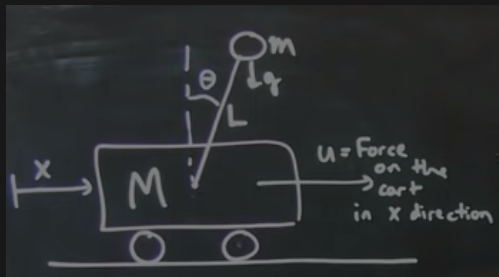
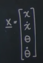
Let us consider a inverted pendulum on a cart having state vector x as below.

This system can be represented by non-linear equation dx/dt = f(x) It can be linearized for fixed points given below.

$$ Θ = 0, π $$

$$ dΘ/dt = 0 $$

$$ x free $$

$$ dx/dt = 0 $$

We can find Jacobian matrix for these fixed points. In case where pendulum is inverted(Θ = π), some of the eigenvalues of matrix A comeout to be positive. To stabalize the pendulum in this position we can use pole placement

---

Pole Placement for the Inverted Pendulum on a Cart

After linearising and including control term we get equation as below. dx/dt = (A - Bk)x Here K is controller vector which manipulates eigenvalues of A - Bk to achieve stability.

In Matlab we can specify eigenvalues and find out vector k. And then we can simulate the system.

Negative eigenvalues will stabalize the system. Increasing the magnitude of eigenvalue will result in faster stabalization. But increasing it beyond certain value the non-linear system dynamics become unstable.

---

LQR Control for the Inverted Pendulum on a Cart

LQR stands for linear quadratic control. It gives us optimal value for matrix k by penalising change in system coordinates and power consumption according to our need.

$$ J = ∫(x^TQx + u^TRu) $$

$$ J = ∫(x^TQx - u^TRkx) $$

Here Q is matrix which represents how much penalty should be given if system deviates from desired state and R represents penalty for using power. Optimal K will be the one which minimizes this quadratic cost function.

In Matlab we can find K using command k = lqr(A, B, Q, R)

---

Full State Esimation

We would like to have full state measurements of system $x$ as then we can find optimal full state feedback controler easily. But we might not have access to full state measurements, then vector of system states becomes y = Cx

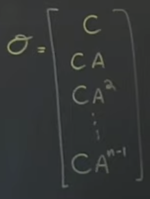
Observability is whether we can estimate full state from measurements y(t) Consider observability matrix as below

If rank(O) = n, system is observable.

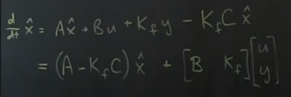
To estimate the full state we need to design a estimator which accepts u and y as input and outputs x̂ which is estimated full state. This estimator itself is a linear dynamical system. It can be represented as

$$ dx̂/dt = Ax̂ + Bu + K_f(y-̂y) $$

$$ ŷ = Cx̂ $$

Here K_f is Kalman filter gain matrix. The term

$$ K_f(y-̂y) $$

updates estimated x̂ based on new values of y.