

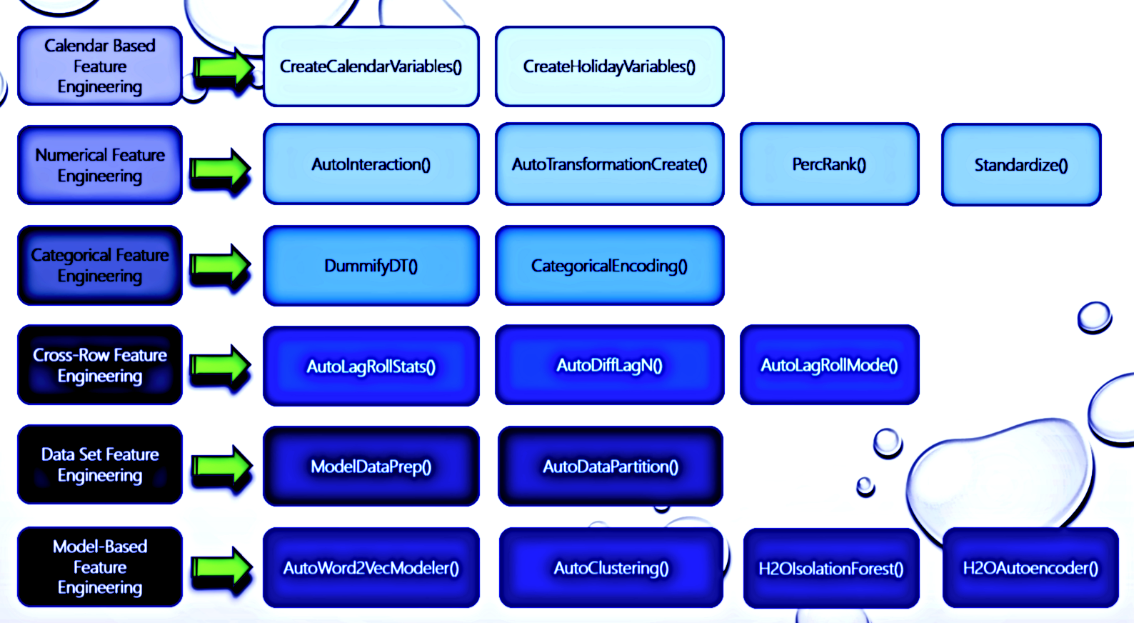
R Optimized Data Engineering Operations
Note: see vignette for examples and parameter definitions
install.packages('bit64')
install.packages('data.table')
install.packages('collapse')
install.packages('timeDate')
install.packages('h2o')
install.packages('Rfast')
install.packages('combinat')
install.packages('nortest')
install.packages('lubridate')
install.packages('fBasics')
devtools::install_github("AdrianAntico/AutoNLP", upgrade = FALSE)- Nested random effects
- Actuarial buhlmann credibility
- Target encoding
- Weight of Evidence
- m-estimator
- poly encode
- backward_difference
- helmert
- All levels
- Partital set of levels
- Numeric transformations
- Interactions
- Calendar variables
- Holiday variables
- Lags and Rolling stats for numeric variables
- Differencing for numeric, date, and categorical variables
- Rolling modes for categorical variables
- Partitioning
- Type conversion for modeling
- Dimensionality reduction
- Clustering
- Word2Vec
- Anomaly detection
Code Example
# Create fake Panel Data----
Count <- 1L
for(Level in LETTERS) {
  datatemp <- AutoQuant::FakeDataGenerator(
    Correlation = 0.75,
    N = 25000L,
    ID = 0L,
    ZIP = 0L,
    FactorCount = 0L,
    AddDate = TRUE,
    Classification = FALSE,
    MultiClass = FALSE)
  datatemp[, Factor1 := eval(Level)]
  if(Count == 1L) {
    data <- data.table::copy(datatemp)
  } else {
    data <- data.table::rbindlist(list(data, data.table::copy(datatemp)))
  }
  Count <- Count + 1L
}

# Add scoring records
data <- Rodeo::AutoLagRollStats(

  # Data
  data                 = data,
  DateColumn           = "DateTime",
  Targets              = "Adrian",
  HierarchyGroups      = NULL,
  IndependentGroups    = c("Factor1"),
  TimeUnitAgg          = "days",
  TimeGroups           = c("days", "weeks", "months", "quarters"),
  TimeBetween          = NULL,
  TimeUnit             = "days",

  # Services
  RollOnLag1           = TRUE,
  Type                 = "Lag",
  SimpleImpute         = TRUE,

  # Calculated Columns
  Lags                 = list("days" = c(seq(1,5,1)), "weeks" = c(seq(1,3,1)), "months" = c(seq(1,2,1)), "quarters" = c(seq(1,2,1))),
  MA_RollWindows       = list("days" = c(seq(1,5,1)), "weeks" = c(seq(1,3,1)), "months" = c(seq(1,2,1)), "quarters" = c(seq(1,2,1))),
  SD_RollWindows       = NULL,
  Skew_RollWindows     = NULL,
  Kurt_RollWindows     = NULL,
  Quantile_RollWindows = NULL,
  Quantiles_Selected   = NULL,
  Debug                = FALSE)
Code Example
# Create fake Panel Data----
Count <- 1L
for(Level in LETTERS) {
  datatemp <- AutoQuant::FakeDataGenerator(
    Correlation = 0.75,
    N = 25000L,
    ID = 0L,
    ZIP = 0L,
    FactorCount = 0L,
    AddDate = TRUE,
    Classification = FALSE,
    MultiClass = FALSE)
  datatemp[, Factor1 := eval(Level)]
  if(Count == 1L) {
    data <- data.table::copy(datatemp)
  } else {
    data <- data.table::rbindlist(list(data, data.table::copy(datatemp)))
  }
  Count <- Count + 1L
}

# Create ID columns to know which records to score
data[, ID := .N:1L, by = "Factor1"]
data.table::set(data, i = which(data[["ID"]] == 2L), j = "ID", value = 1L)

# Score records
data <- Rodeo::AutoLagRollStatsScoring(

  # Data
  data                 = data,
  RowNumsID            = "ID",
  RowNumsKeep          = 1,
  DateColumn           = "DateTime",
  Targets              = "Adrian",
  HierarchyGroups      = c("Store","Dept"),
  IndependentGroups    = NULL,

  # Services
  TimeBetween          = NULL,
  TimeGroups           = c("days", "weeks", "months"),
  TimeUnit             = "day",
  TimeUnitAgg          = "day",
  RollOnLag1           = TRUE,
  Type                 = "Lag",
  SimpleImpute         = TRUE,

  # Calculated Columns
  Lags                  = list("days" = c(seq(1,5,1)), "weeks" = c(seq(1,3,1)), "months" = c(seq(1,2,1))),
  MA_RollWindows        = list("days" = c(seq(1,5,1)), "weeks" = c(seq(1,3,1)), "months" = c(seq(1,2,1))),
  SD_RollWindows        = list("days" = c(seq(1,5,1)), "weeks" = c(seq(1,3,1)), "months" = c(seq(1,2,1))),
  Skew_RollWindows      = list("days" = c(seq(1,5,1)), "weeks" = c(seq(1,3,1)), "months" = c(seq(1,2,1))),
  Kurt_RollWindows      = list("days" = c(seq(1,5,1)), "weeks" = c(seq(1,3,1)), "months" = c(seq(1,2,1))),
  Quantile_RollWindows  = list("days" = c(seq(1,5,1)), "weeks" = c(seq(1,3,1)), "months" = c(seq(1,2,1))),
  Quantiles_Selected    = c("q5","q10","q95"),
  Debug                 = FALSE)
Function Description
AutoLagRollStats() builds lags and rolling statistics by grouping variables and their interactions along with multiple different time aggregations if selected. Rolling stats include mean, sd, skewness, kurtosis, and the 5th - 95th percentiles. This function was inspired by the distributed lag modeling framework but I wanted to use it for time series analysis as well and really generalize it as much as possible. The beauty of this function is inspired by analyzing whether a baseball player will get a basehit or more in his next at bat. One easy way to get a better idea of the likelihood is to look at his batting average and his career batting average. However, players go into hot streaks and slumps. How do we account for that? Well, in comes the functions here. You look at the batting average over the last N to N+x at bats, for various N and x. I keep going though - I want the same windows for calculating the players standard deviation, skewness, kurtosis, and various quantiles over those time windows. I also want to look at all those measure but by using weekly data - as in, over the last N weeks, pull in those stats too.
AutoLagRollStatsScoring() builds the above features for a partial set of records in a data set. The function is extremely useful as it can compute these feature vectors at a significantly faster rate than the non scoring version which comes in handy for scoring ML models. If you can find a way to make it faster, let me know.
Code Example
# NO GROUPING CASE: Create fake Panel Data----
Count <- 1L
for(Level in LETTERS) {
  datatemp <- AutoQuant::FakeDataGenerator(
    Correlation = 0.75,
    N = 25000L,
    ID = 0L,
    ZIP = 0L,
    FactorCount = 2L,
    AddDate = TRUE,
    Classification = FALSE,
    MultiClass = FALSE)
  datatemp[, Factor1 := eval(Level)]
  if(Count == 1L) {
    data <- data.table::copy(datatemp)
  } else {
    data <- data.table::rbindlist(
      list(data, data.table::copy(datatemp)))
  }
  Count <- Count + 1L
}

# NO GROUPING CASE: Create rolling modes for categorical features
data <- Rodeo::AutoLagRollMode(
  data,
  Lags           = seq(1,5,1),
  ModePeriods    = seq(2,5,1),
  Targets        = c("Factor_1"),
  GroupingVars   = NULL,
  SortDateName   = "DateTime",
  WindowingLag   = 1,
  Type           = "Lag",
  SimpleImpute   = TRUE)

# GROUPING CASE: Create fake Panel Data----
Count <- 1L
for(Level in LETTERS) {
  datatemp <- AutoQuant::FakeDataGenerator(
    Correlation = 0.75,
    N = 25000L,
    ID = 0L,
    ZIP = 0L,
    FactorCount = 2L,
    AddDate = TRUE,
    Classification = FALSE,
    MultiClass = FALSE)
  datatemp[, Factor1 := eval(Level)]
  if(Count == 1L) {
    data <- data.table::copy(datatemp)
  } else {
    data <- data.table::rbindlist(
      list(data, data.table::copy(datatemp)))
  }
  Count <- Count + 1L
}

# GROUPING CASE: Create rolling modes for categorical features
data <- Rodeo::AutoLagRollMode(
  data,
  Lags           = seq(1,5,1),
  ModePeriods    = seq(2,5,1),
  Targets        = c("Factor_1"),
  GroupingVars   = "Factor_2",
  SortDateName   = "DateTime",
  WindowingLag   = 1,
  Type           = "Lag",
  SimpleImpute   = TRUE)
Function Description
AutoLagRollMode() Generate lags and rolling modes for categorical variables
Code Example
##############################
# Current minus lag1
##############################

# Create fake data
data <- AutoQuant::FakeDataGenerator(
  Correlation = 0.70,
  N = 50000,
  ID = 2L,
  FactorCount = 3L,
  AddDate = TRUE,
  ZIP = 0L,
  TimeSeries = FALSE,
  ChainLadderData = FALSE,
  Classification = FALSE,
  MultiClass = FALSE)

# Store Cols to diff
Cols <- names(data)[which(unlist(data[, lapply(.SD, is.numeric)]))]

# Clean data before running AutoDiffLagN
data <- Rodeo::ModelDataPrep(
  data = data,
  Impute = FALSE,
  CharToFactor = FALSE,
  FactorToChar = TRUE)

# Run function
data <- Rodeo::AutoDiffLagN(
  data,
  DateVariable = "DateTime",
  GroupVariables = c("Factor_2"),
  DiffVariables = Cols,
  DiffDateVariables = "DateTime",
  DiffGroupVariables = "Factor_1",
  NLag1 = 0,
  NLag2 = 1,
  Sort = TRUE,
  RemoveNA = TRUE)

##############################
# lag1 minus lag3
##############################

# Create fake data
data <- AutoQuant::FakeDataGenerator(
  Correlation = 0.70,
  N = 50000,
  ID = 2L,
  FactorCount = 3L,
  AddDate = TRUE,
  ZIP = 0L,
  TimeSeries = FALSE,
  ChainLadderData = FALSE,
  Classification = FALSE,
  MultiClass = FALSE)

# Store Cols to diff
Cols <- names(data)[which(unlist(data[, lapply(.SD, is.numeric)]))]

# Clean data before running AutoDiffLagN
data <- Rodeo::ModelDataPrep(
  data = data,
  Impute = FALSE,
  CharToFactor = FALSE,
  FactorToChar = TRUE)

# Run function
data <- Rodeo::AutoDiffLagN(
  data,
  DateVariable = "DateTime",
  GroupVariables = c("Factor_2"),
  DiffVariables = Cols,
  DiffDateVariables = "DateTime",
  DiffGroupVariables = "Factor_1",
  NLag1 = 1,
  NLag2 = 3,
  Sort = TRUE,
  RemoveNA = TRUE)
Function Description
AutoDiffLagN() Generate differences for numeric columns, date columns, and categorical columns, by groups. You can specify NLag1 and NLag2 to generate the diffs based on any two time periods.
Code Example
#########################################
# Feature Engineering for Model Training
#########################################

# Create fake data
data <- AutoQuant::FakeDataGenerator(
  Correlation = 0.70,
  N = 50000,
  ID = 2L,
  FactorCount = 2L,
  AddDate = TRUE,
  ZIP = 0L,
  TimeSeries = FALSE,
  ChainLadderData = FALSE,
  Classification = FALSE,
  MultiClass = FALSE)

# Print number of columns
print(ncol(data))

# Store names of numeric and integer cols
Cols <-names(data)[c(which(unlist(lapply(data, is.numeric))),
                     which(unlist(lapply(data, is.integer))))]

# Model Training Feature Engineering
system.time(data <- Rodeo::AutoInteraction(
  data = data,
  NumericVars = Cols,
  InteractionDepth = 4,
  Center = TRUE,
  Scale = TRUE,
  SkipCols = NULL,
  Scoring = FALSE,
  File = getwd()))

# user  system elapsed
# 0.32    0.22    0.53

# Print number of columns
print(ncol(data))
# 16

########################################
# Feature Engineering for Model Scoring
########################################

# Create fake data
data <- AutoQuant::FakeDataGenerator(
  Correlation = 0.70,
  N = 50000,
  ID = 2L,
  FactorCount = 2L,
  AddDate = TRUE,
  ZIP = 0L,
  TimeSeries = FALSE,
  ChainLadderData = FALSE,
  Classification = FALSE,
  MultiClass = FALSE)

# Print number of columns
print(ncol(data))
# 16

# Reduce to single row to mock a scoring scenario
data <- data[1L]

# Model Scoring Feature Engineering
system.time(data <- Rodeo::AutoInteraction(
  data = data,
  NumericVars = names(data)[
    c(which(unlist(lapply(data, is.numeric))),
      which(unlist(lapply(data, is.integer))))],
  InteractionDepth = 4,
  Center = TRUE,
  Scale = TRUE,
  SkipCols = NULL,
  Scoring = TRUE,
  File = file.path(getwd(), "Standardize.Rdata")))

# user  system elapsed
# 0.19    0.00    0.19

# Print number of columns
print(ncol(data))
# 1095
Function Description
AutoInteraction() will build out any number of interactions you want for numeric variables. You supply a character vector of numeric or integer column names, along with the names of any numeric columns you want to skip (including the interaction column names) and the interactions will be automatically created for you. For example, if you want a 4th degree interaction from 10 numeric columns, you will have 10 C 2, 10 C 3, and 10 C 4 columns created. Now, let's say you build all those features and decide you don't want all 10 features to be included. Remove the feature name from the NumericVars character vector. Now, let's say you modeled all of the interaction features and want to remove the ones will the lowest scores on the variable importance list. Grab the names and run the interaction function again except this time supply those poor performing interaction column names to the SkipCols argument and they will be ignored. Now, if you want to interact any categorical variable with a numeric variable, you'll have to dummify the categorical variable first and then include the level specific dummy variable column names to the NumericVars character vector argument. If you set Center and Scale to TRUE then the interaction multiplication won't create huge numbers.
Code Example
# Create fake data
data <- AutoQuant::FakeDataGenerator(
  Correlation = 0.70,
  N = 1000L,
  ID = 2L,
  FactorCount = 2L,
  AddDate = TRUE,
  AddComment = TRUE,
  ZIP = 2L,
  TimeSeries = FALSE,
  ChainLadderData = FALSE,
  Classification = FALSE,
  MultiClass = FALSE)

# Create Model and Vectors
data <- Rodeo::AutoWord2VecModeler(
  data,
  BuildType = "individual",
  stringCol = c("Comment"),
  KeepStringCol = FALSE,
  ModelID = "Model_1",
  model_path = getwd(),
  vects = 10,
  MinWords = 1,
  WindowSize = 1,
  Epochs = 25,
  SaveModel = "standard",
  Threads = max(1,parallel::detectCores()-2),
  MaxMemory = "28G")

# Remove data
rm(data)

# Create fake data for mock scoring
data <- AutoQuant::FakeDataGenerator(
  Correlation = 0.70,
  N = 1000L,
  ID = 2L,
  FactorCount = 2L,
  AddDate = TRUE,
  AddComment = TRUE,
  ZIP = 2L,
  TimeSeries = FALSE,
  ChainLadderData = FALSE,
  Classification = FALSE,
  MultiClass = FALSE)

# Create vectors for scoring
data <- Rodeo::AutoWord2VecScoring(
  data,
  BuildType = "individual",
  ModelObject = NULL,
  ModelID = "Model_1",
  model_path = getwd(),
  stringCol = "Comment",
  KeepStringCol = FALSE,
  H2OStartUp = TRUE,
  H2OShutdown = TRUE,
  Threads = max(1L, parallel::detectCores() - 2L),
  MaxMemory = "28G")
Function Description
AutoWord2VecModeler() generates a specified number of vectors (word2vec) for each column of text data in your data set that you specify and it will save the models if you specify for re-creating them later in a model scoring process. You can choose to build individual models for each column or one model for all your columns. If you need to run several models for groups of text variables you can run the function several times.
AutoWord2VecScoring() this is for generating word2vec vectors for model scoring situations. The function will load the model, create the transformations, and merge them onto the source data.table just like the training version does.
Code Example
# Create fake data with 10 categorical
data <- AutoQuant::FakeDataGenerator(
  Correlation = 0.85,
  N = 1000000,
  ID = 2L,
  ZIP = 0,
  FactorCount = 10L,
  AddDate = FALSE,
  Classification = TRUE,
  MultiClass = FALSE)

# Take your pick
Meth <- c('credibility',
          'woe',
          'target_encoding',
          'poly_encode',
          'backward_difference',
          'helmert')

# Pass to function
MethNum <- 1

# Mock test data with same factor levels
test <- data.table::copy(data)

# Run in Train Mode
data <- Rodeo::CategoricalEncoding(
  data = data,
  ML_Type = "classification",
  GroupVariables = paste0("Factor_", 1:10),
  TargetVariable = "Adrian",
  Method = Meth[MethNum],
  SavePath = getwd(),
  Scoring = FALSE,
  ReturnFactorLevelList = FALSE,
  SupplyFactorLevelList = NULL,
  KeepOriginalFactors = FALSE)

# View results
print(data)

# Run in Score Mode by pulling in the csv's
test <- Rodeo::CategoricalEncoding(
  data = data,
  ML_Type = "classification",
  GroupVariables = paste0("Factor_", 1:10),
  TargetVariable = "Adrian",
  Method = Meth[MethNum],
  SavePath = getwd(),
  Scoring = TRUE,
  ImputeValueScoring = 222,
  ReturnFactorLevelList = FALSE,
  SupplyFactorLevelList = NULL,
  KeepOriginalFactors = FALSE)
}
Function Description
CategoricalEncoding() enables you to convert your categorical variables into numeric variables in seven different ways. You can choose from m_estimator, credibility (a.k.a. James Stein), weight of evidence, target encoding, poly encoding, backward difference encoding, and helmert encoding. You can run the function for training data and for scoring situations (on demand or batch). For scoring, you can choose to supply an imputation value for new levels that may show up or you can manage them somewhere else in the pipeline. For scoring, you have two options: during the training run you can save the metadata to file by supplying a path to SavePath or you can have the metadata returned by setting ReturnFactorLevelList to TRUE and in scoring your can either have the files pulled from file using the SavePath argument and the function will take care of the rest or you can supply the ReturnFactorLevelList to the SupplyFactorLevelList argument and the function will take care of the rest.
Code Example
############################
# Training
############################

# Create simulated data
data <- AutoQuant::FakeDataGenerator(
  Correlation = 0.70,
  N = 1000L,
  ID = 2L,
  FactorCount = 2L,
  AddDate = TRUE,
  AddComment = FALSE,
  ZIP = 2L,
  TimeSeries = FALSE,
  ChainLadderData = FALSE,
  Classification = FALSE,
  MultiClass = FALSE)

# Run algo
Output <- Rodeo::H2OAutoencoder(

  # Select the service
  AnomalyDetection = TRUE,
  DimensionReduction = TRUE,

  # Data related args
  data = data,
  ValidationData = NULL,
  Features = names(data)[2L:(ncol(data)-1L)],
  per_feature = FALSE,
  RemoveFeatures = TRUE,
  ModelID = "TestModel",
  model_path = getwd(),

  # H2O Environment
  NThreads = max(1L, parallel::detectCores()-2L),
  MaxMem = "28G",
  H2OStart = TRUE,
  H2OShutdown = TRUE,

  # H2O ML Args
  LayerStructure = NULL,
  ReturnLayer = 4L,
  Activation = "Tanh",
  Epochs = 5L,
  L2 = 0.10,
  ElasticAveraging = TRUE,
  ElasticAveragingMovingRate = 0.90,
  ElasticAveragingRegularization = 0.001)

# Inspect output
data <- Output$Data
Model <- Output$Model

# If ValidationData is not null
ValidationData <- Output$ValidationData

############################
# Scoring
############################

# Create simulated data
data <- AutoQuant::FakeDataGenerator(
  Correlation = 0.70,
  N = 1000L,
  ID = 2L,
  FactorCount = 2L,
  AddDate = TRUE,
  AddComment = FALSE,
  ZIP = 2L,
  TimeSeries = FALSE,
  ChainLadderData = FALSE,
  Classification = FALSE,
  MultiClass = FALSE)

# Run algo
data <- Rodeo::H2OAutoencoderScoring(

  # Select the service
  AnomalyDetection = TRUE,
  DimensionReduction = TRUE,

  # Data related args
  data = data,
  Features = names(data)[2L:ncol(data)],
  RemoveFeatures = TRUE,
  ModelObject = NULL,
  ModelID = "TestModel",
  model_path = getwd(),

  # H2O args
  NThreads = max(1L, parallel::detectCores()-2L),
  MaxMem = "28G",
  H2OStart = TRUE,
  H2OShutdown = TRUE,
  ReturnLayer = 4L,
  per_feature = FALSE)
Function Description
H2OAutoencoder() Use for dimension reduction and anomaly detection
H2OAutoencoderScoring() Use for dimension reduction and anomaly detection scoring
Code Example
# Create simulated data
data <- AutoQuant::FakeDataGenerator(
  Correlation = 0.70,
  N = 50000,
  ID = 2L,
  FactorCount = 2L,
  AddDate = TRUE,
  ZIP = 0L,
  TimeSeries = FALSE,
  ChainLadderData = FALSE,
  Classification = FALSE,
  MultiClass = FALSE)

# Run algo
data <- Rodeo::H2OIsolationForest(
  data,
  Features = names(data)[2L:ncol(data)],
  IDcols = c("Adrian", "IDcol_1", "IDcol_2"),
  ModelID = "Adrian",
  SavePath = getwd(),
  Threshold = 0.95,
  MaxMem = "28G",
  NThreads = -1,
  NTrees = 100,
  SampleRate = (sqrt(5)-1)/2,
  MaxDepth = 8,
  MinRows = 1,
  ColSampleRate = 1,
  ColSampleRatePerLevel = 1,
  ColSampleRatePerTree = 1,
  CategoricalEncoding = c("AUTO"),
  Debug = TRUE)

# Remove output from data and then score
data[, eval(names(data)[17:ncol(data)]) := NULL]

# Run algo
Outliers <- Rodeo::H2OIsolationForestScoring(
  data,
  Features = names(data)[2:ncol(data)],
  IDcols = c("Adrian", "IDcol_1", "IDcol_2"),
  H2OStart = TRUE,
  H2OShutdown = TRUE,
  ModelID = "TestModel",
  SavePath = getwd(),
  Threshold = 0.95,
  MaxMem = "28G",
  NThreads = -1,
  Debug = FALSE)
Function Description
H2OIsolationForecast() Anomaly detection and feature engineering using H2O Isolation Forest. A model is built, your training data is scored, and the model is saved to file for later use in scoring environments with H2OIsolationForestScoring()
H2OIsolationForecastScoring() Scoring function
Code Example
#########################
# Training Setup
#########################

# Create fake data
data <- AutoQuant::FakeDataGenerator(
  Correlation = 0.85,
  N = 1000,
  ID = 2,
  ZIP = 0,
  AddDate = TRUE,
  Classification = FALSE,
  MultiClass = FALSE)

# Run function
data <- Rodeo::AutoClustering(
  data,
  FeatureColumns = names(data)[2:(ncol(data)-1)],
  ModelID = "TestModel",
  SavePath = getwd(),
  NThreads = 8,
  MaxMemory = "28G",
  MaxClusters = 50,
  ClusterMetric = "totss",
  RunDimReduction = TRUE,
  ShrinkRate = (sqrt(5) - 1) / 2,
  Epochs = 5L,
  L2_Reg = 0.10,
  ElasticAveraging = TRUE,
  ElasticAveragingMovingRate = 0.90,
  ElasticAveragingRegularization = 0.001)

#########################
# Scoring Setup
#########################

Sys.sleep(10)

# Create fake data
data <- AutoQuant::FakeDataGenerator(
  Correlation = 0.85,
  N = 1000,
  ID = 2,
  ZIP = 0,
  AddDate = TRUE,
  Classification = FALSE,
  MultiClass = FALSE)

# Run function
data <- Rodeo::AutoClusteringScoring(
  data,
  FeatureColumns = names(data)[2:(ncol(data)-1)],
  ModelID = "TestModel",
  SavePath = getwd(),
  NThreads = 8,
  MaxMemory = "28G",
  DimReduction = TRUE)
Function Description
AutoClustering() Generates a single column and merges it onto your data. You can have an autoencoder ran to reduce the dimension size before running the KMeans grid tuning operation. If you provide a directory path, the models will be saved and can be used later in scoring enviroments. I find that I utilize clustering more often for feature engineering that unsupervised learning which is why I put the code example and description here. The function utilizes H2O under the hood with their KMeans algo for the clustering and their deep learning algo for the dimensionality reduction.
Code Example
# Create fake data with a Date column----
data <- AutoQuant::FakeDataGenerator(
  Correlation = 0.75,
  N = 25000L,
  ID = 2L,
  ZIP = 0L,
  FactorCount = 4L,
  AddDate = TRUE,
  Classification = FALSE,
  MultiClass = FALSE)
for(i in seq_len(20L)) {
  print(i)
  data <- data.table::rbindlist(list(data, AutoQuant::FakeDataGenerator(
    Correlation = 0.75,
    N = 25000L,
    ID = 2L,
    ZIP = 0L,
    FactorCount = 4L,
    AddDate = TRUE,
    Classification = FALSE,
    MultiClass = FALSE)))
}

# Create calendar variables - automatically excludes the second, minute, and hour selections since
#   it is not timestamp data
runtime <- system.time(
  data <- Rodeo::CreateCalendarVariables(
    data = data,
    DateCols = "DateTime",
    AsFactor = FALSE,
    TimeUnits = c("second", "minute", "hour", "wday", "mday", "yday", "week", "isoweek", "wom", "month", "quarter", "year")))
head(data)
print(runtime)
Function Description
CreateCalendarVariables() This functions creates numerical columns based on the date columns you supply such as second, minute, hour, week day, day of month, day of year, week, isoweek, wom, month, quarter, and year.
Code Example
# Create fake data with a Date----
data <- AutoQuant::FakeDataGenerator(
  Correlation = 0.75,
  N = 25000L,
  ID = 2L,
  ZIP = 0L,
  FactorCount = 4L,
  AddDate = TRUE,
  Classification = FALSE,
  MultiClass = FALSE)
for(i in seq_len(20L)) {
  print(i)
  data <- data.table::rbindlist(list(data, AutoQuant::FakeDataGenerator(
    Correlation = 0.75,
    N = 25000L,
    ID = 2L,
    ZIP = 0L,
    FactorCount = 4L,
    AddDate = TRUE,
    Classification = FALSE,
    MultiClass = FALSE)))
}
# Run function and time it
runtime <- system.time(
  data <- CreateHolidayVariables(
    data,
    DateCols = "DateTime",
    LookbackDays = 7,
    HolidayGroups = c("USPublicHolidays","EasterGroup","ChristmasGroup","OtherEcclesticalFeasts"),
    Holidays = NULL
    Print = FALSE))
head(data)
print(runtime)
Function Description
CreateHolidayVariable()
This function counts up the number of specified holidays between the current record time stamp and the previous record time stamp, by group as well if specified.
Code Example
# Create fake data with 10 categorical columns
data <- AutoQuant::FakeDataGenerator(
  Correlation = 0.85,
  N = 25000,
  ID = 2L,
  ZIP = 0,
  FactorCount = 10L,
  AddDate = FALSE,
  Classification = FALSE,
  MultiClass = FALSE)

# Create dummy variables
data <- DummifyDT(
  data = data,
  cols = c("Factor_1",
           "Factor_2",
           "Factor_3",
           "Factor_4",
           "Factor_5",
           "Factor_6",
           "Factor_8",
           "Factor_9",
           "Factor_10"),
  TopN = c(rep(3,9)),
  KeepFactorCols = TRUE,
  OneHot = FALSE,
  SaveFactorLevels = TRUE,
  SavePath = getwd(),
  ImportFactorLevels = FALSE,
  FactorLevelsList = NULL,
  ClustScore = FALSE,
  ReturnFactorLevels = FALSE)

# Create Fake Data for Scoring Replication
data <- AutoQuant::FakeDataGenerator(
  Correlation = 0.85,
  N = 25000,
  ID = 2L,
  ZIP = 0,
  FactorCount = 10L,
  AddDate = FALSE,
  Classification = FALSE,
  MultiClass = FALSE)

# Scoring Version (imports csv's to generate matching levels and ordering)
data <- Rodeo::DummifyDT(
  data = data,
  cols = c("Factor_1",
           "Factor_2",
           "Factor_3",
           "Factor_4",
           "Factor_5",
           "Factor_6",
           "Factor_8",
           "Factor_9",
           "Factor_10"),
  TopN = c(rep(3,9)),
  KeepFactorCols = TRUE,
  OneHot = FALSE,
  SaveFactorLevels = TRUE,
  SavePath = getwd(),
  ImportFactorLevels = TRUE,
  FactorLevelsList = NULL,
  ClustScore = FALSE,
  ReturnFactorLevels = FALSE)
Function Description
DummifyDT() This function is used in the AutoXGBoost__() suite of modeling functions to manage categorical variables in your training, validation, and test sets. This function rapidly dichotomizes categorical columns in a data.table (N+1 columns for N levels using one hot encoding or N columns for N levels otherwise). Several other arguments exist for outputting and saving factor levels. This is useful in model training, validating, and scoring processes.
Code Example
# Create fake data
data <- AutoQuant::FakeDataGenerator(
  Correlation = 0.85,
  N = 1000,
  ID = 2,
  ZIP = 0,
  AddDate = FALSE,
  Classification = FALSE,
  MultiClass = FALSE)

# Run data partitioning function
dataSets <- Rodeo::AutoDataPartition(
  data,
  NumDataSets = 3L,
  Ratios = c(0.70,0.20,0.10),
  PartitionType = "random",
  StratifyColumnNames = NULL,
  TimeColumnName = NULL)

# Collect data
TrainData <- dataSets$TrainData
ValidationData <- dataSets$ValidationData
TestData <- dataSets$TestData
Function Description
AutoDataPartition() is designed to achieve a few things that standard data partitioning processes or functions don't handle. First, you can choose to build any number of partitioned data sets beyond the standard train, validate, and test data sets. Second, you can choose between random sampling to split your data or you can choose a time-based partitioning. Third, for the random partitioning, you can specify a stratification columns in your data to stratify by in order to ensure a proper split amongst your categorical features (E.g. think MultiClass targets). Lastly, it's 100% data.table so it will run fast and with low memory overhead.
Code Example
# Create fake data
data <- AutoQuant::FakeDataGenerator(
  Correlation = 0.75,
  N = 250000L,
  ID = 2L,
  ZIP = 0L,
  FactorCount = 6L,
  AddDate = TRUE,
  AddComment = FALSE,
  TimeSeries = FALSE,
  AddDate = TRUE,
  Classification = FALSE,
  MultiClass = FALSE)

# Check column types
str(data)

# RUn function
data <- Rodeo::ModelDataPrep(
  data,
  Impute = TRUE,
  CharToFactor = FALSE,
  FactorToChar = TRUE,
  IntToNumeric = TRUE,
  LogicalToBinary = FALSE,
  DateToChar = FALSE,
  RemoveDates = TRUE,
  MissFactor = "0",
  MissNum = -1,
  IgnoreCols = c("Factor_1"))

# Check column types
str(data)
Function Description
ModelDataPrep() This function will loop through every column in your data and apply a variety of functions based on argument settings. For all columns not ignored, these tasks include:
- Character type to Factor type converstion
- Factor type to Character type conversion
- Constant value imputation for numeric and categorical columns
- Integer type to Numeric type conversion
- Date type to Character type conversion
- Remove date columns
- Ignore specified columns
Function Description
AutoTransformationCreate() is a function for automatically identifying the optimal transformations for numeric features and transforming them once identified. This function will loop through your selected transformation options (YeoJohnson, BoxCox, Asinh, Log, LogPlus1, Sqrt, along with Asin and Logit for proportion data) and find the one that produces the best fit to a normal distribution. It then generates the transformation and collects the metadata information for use in the AutoTransformationScore() function, either by returning the objects or saving them to file.
AutoTransformationScore() is a the compliment function to AutoTransformationCreate(). Automatically apply or inverse the transformations you identified in AutoTransformationCreate() to other data sets. This is useful for applying transformations to your validation and test data sets for modeling, which is done automatically for you if you specify.