Building a powerful image classifier, using only very few training examples --just a few hundred or thousand pictures from each class you want to be able to recognize.
- Python 3.0+
- ML Lib.(numpy, matplotlib, pandas, scikit learn)
- TensorFlow
- Keras
CNNs are made up of neurons that have learnable weights and biases. Each neuron receives some inputs, performs a dot product and optionally follows it with a non-linearity. The whole network still expresses a single differentiable score function: from the raw image pixels on one end to class scores at the other. And they still have a loss function (e.g. SVM/Softmax) on the last (fully-connected) layer and all the tips/tricks we developed for learning regular Neural Networks still apply.
As we described above, a simple ConvNet is a sequence of layers, and every layer of a ConvNet transforms one volume of activations to another through a differentiable function. We use three main types of layers to build ConvNet architectures: Convolutional Layer, Pooling Layer, and Fully-Connected Layer (exactly as seen in regular Neural Networks). We will stack these layers to form a full ConvNet architecture.
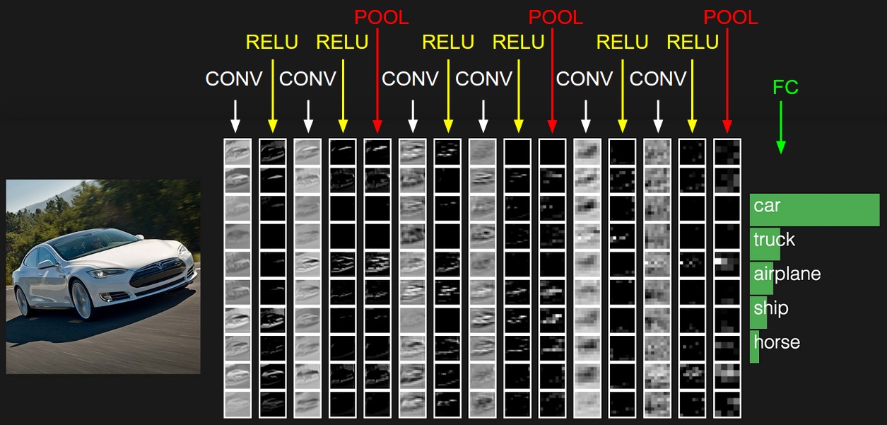
Example Architecture: Overview. We will go into more details below, but a simple ConvNet for CIFAR-10 classification could have the architecture [INPUT - CONV - RELU - POOL - FC]. In more detail:
- INPUT [32x32x3] will hold the raw pixel values of the image, in this case an image of width 32, height 32, and with three color channels R,G,B.
- CONV layer will compute the output of neurons that are connected to local regions in the input, each computing a dot product between their weights and a small region they are connected to in the input volume. This may result in volume such as [32x32x12] if we decided to use 12 filters.
- RELU layer will apply an elementwise activation function, such as the max(0,x)max(0,x) thresholding at zero. This leaves the size of the volume unchanged ([32x32x12]). POOL layer will perform a downsampling operation along the spatial dimensions (width, height), resulting in volume such as [16x16x12].
- FC (i.e. fully-connected) layer will compute the class scores, resulting in volume of size [1x1x10], where each of the 10 numbers correspond to a class score, such as among the 10 categories of CIFAR-10. As with ordinary Neural Networks and as the name implies, each neuron in this layer will be connected to all the numbers in the previous volume.
In this way, ConvNets transform the original image layer by layer from the original pixel values to the final class scores. Note that some layers contain parameters and other don’t. In particular, the CONV/FC layers perform transformations that are a function of not only the activations in the input volume, but also of the parameters (the weights and biases of the neurons). On the other hand, the RELU/POOL layers will implement a fixed function. The parameters in the CONV/FC layers will be trained with gradient descent so that the class scores that the ConvNet computes are consistent with the labels in the training set for each image.
In Summary:
A ConvNet architecture is in the simplest case a list of Layers that transform the image volume into an output volume (e.g. holding the class scores)
- There are a few distinct types of Layers (e.g. CONV/FC/RELU/POOL are by far the most popular)
- Each Layer accepts an input 3D volume and transforms it to an output 3D volume through a differentiable function
- Each Layer may or may not have parameters (e.g. CONV/FC do, RELU/POOL don’t)
- Each Layer may or may not have additional hyperparameters (e.g. CONV/FC/POOL do, RELU doesn’t)
Data can be downloaded at: https://www.kaggle.com/c/dogs-vs-cats/data All you need is the train set
We will go over the following options:
- Training a small network from scratch (as a baseline)
- Using the bottleneck features of a pre-trained network
- Fine-tuning the top layers of a pre-trained network
Data Loading
##Updated to Keras 2.0
import os
import numpy as np
from keras.models import Sequential
from keras.layers import Activation, Dropout, Flatten, Dense
from keras.preprocessing.image import ImageDataGenerator
from keras.layers import Convolution2D, MaxPooling2D, ZeroPadding2D
from keras import optimizers
from keras import applications
from keras.models import Model
#Using TensorFlow backend.

# dimensions of our images.
img_width, img_height = 150, 150

train_data_dir = 'data/train'
validation_data_dir = 'data/validation'
Import
##preprocessing
# used to rescale the pixel values from [0, 255] to [0, 1] interval
datagen = ImageDataGenerator(rescale=1./255)
batch_size = 32

# automagically retrieve images and their classes for train and validation sets
train_generator = datagen.flow_from_directory(
       train_data_dir,
       target_size=(img_width, img_height),
       batch_size=batch_size,
       class_mode='binary')

validation_generator = datagen.flow_from_directory(
       validation_data_dir,
       target_size=(img_width, img_height),
       batch_size=batch_size,
       class_mode='binary')
Small Conv Net Model architecture definition
# a simple stack of 3 convolution layers with a ReLU activation and followed by max-pooling layers.
model = Sequential()
model.add(Convolution2D(32, (3, 3), input_shape=(img_width, img_height,3)))
model.add(Activation('relu'))
model.add(MaxPooling2D(pool_size=(2, 2)))

model.add(Convolution2D(32, (3, 3)))
model.add(Activation('relu'))
model.add(MaxPooling2D(pool_size=(2, 2)))

model.add(Convolution2D(64, (3, 3)))
model.add(Activation('relu'))
model.add(MaxPooling2D(pool_size=(2, 2)))

model.add(Flatten())
model.add(Dense(64))
model.add(Activation('relu'))
model.add(Dropout(0.5))
model.add(Dense(1))
model.add(Activation('sigmoid'))

model.compile(loss='binary_crossentropy',
              optimizer='rmsprop',
              metrics=['accuracy'])
Training
epochs = 30
train_samples = 2048
validation_samples = 832
model.fit_generator(
        train_generator,
        steps_per_epoch=train_samples // batch_size,
        epochs=epochs,
        validation_data=validation_generator,
        validation_steps=validation_samples// batch_size,)
Evaluating on validation set
model.evaluate_generator(validation_generator, validation_samples)
Data augmentation for improving the model
By applying random transformation to our train set, we artificially enhance our dataset with new unseen images. This will hopefully reduce overfitting and allows better generalization capability for our network.
train_datagen_augmented = ImageDataGenerator(
        rescale=1./255,        # normalize pixel values to [0,1]
        shear_range=0.2,       # randomly applies shearing transformation
        zoom_range=0.2,        # randomly applies shearing transformation
        horizontal_flip=True)  # randomly flip the images

# same code as before
train_generator_augmented = train_datagen_augmented.flow_from_directory(
        train_data_dir,
        target_size=(img_width, img_height),
        batch_size=batch_size,
        class_mode='binary')

 model.fit_generator(
        train_generator_augmented,
        steps_per_epoch=train_samples // batch_size,
        epochs=epochs,
        validation_data=validation_generator,
        validation_steps=validation_samples // batch_size,)
Evaluating on validation set Computing loss and accuracy :
model.evaluate_generator(validation_generator, validation_samples)
The process of training a convolutionnal neural network can be very time-consuming and require a lot of data. We can go beyond the previous models in terms of performance and efficiency by using a general-purpose, pre-trained image classifier. This example uses VGG16, a model trained on the ImageNet dataset - which contains millions of images classified in 1000 categories.
On top of it, we add a small multi-layer perceptron and we train it on our dataset. We are using VGG16 + small MLP
Available models in Keras Models for image classification with weights trained on ImageNet:
- Xception
- VGG16
- VGG19
- ResNet50
- InceptionV3
- InceptionResNetV2
- MobileNet
- DenseNet
- NASNet
model_vgg = applications.VGG16(include_top=False, weights='imagenet')
Using the VGG16 model to process samples
        train_data_dir,
        target_size=(img_width, img_height),
        batch_size=batch_size,
        class_mode=None,
        shuffle=False)

validation_generator_bottleneck = datagen.flow_from_directory(
        validation_data_dir,
        target_size=(img_width, img_height),
        batch_size=batch_size,
        class_mode=None,
        shuffle=False)
bottleneck_features_train = model_vgg.predict_generator(train_generator_bottleneck, train_samples // batch_size)
np.save(open('models/bottleneck_features_train.npy', 'wb'), bottleneck_features_train)

bottleneck_features_validation = model_vgg.predict_generator(validation_generator_bottleneck, validation_samples // batch_size)
np.save(open('models/bottleneck_features_validation.npy', 'wb'), bottleneck_features_validation)

#Now we can load it...

train_data = np.load(open('models/bottleneck_features_train.npy', 'rb'))
train_labels = np.array([0] * (train_samples // 2) + [1] * (train_samples // 2))

validation_data = np.load(open('models/bottleneck_features_validation.npy', 'rb'))
validation_labels = np.array([0] * (validation_samples // 2) + [1] * (validation_samples // 2))


#And define and train the custom fully connected neural network :

model_top = Sequential()
model_top.add(Flatten(input_shape=train_data.shape[1:]))
model_top.add(Dense(256, activation='relu'))
model_top.add(Dropout(0.5))
model_top.add(Dense(1, activation='sigmoid'))

model_top.compile(optimizer='rmsprop', loss='binary_crossentropy', metrics=['accuracy'])

model_top.fit(train_data, train_labels,
        epochs=epochs,
        batch_size=batch_size,
        validation_data=(validation_data, validation_labels))
Bottleneck model evaluation Loss and accuracy :
model_top.evaluate(validation_data, validation_labels)