How much of your Neural Network’s Prediction can be Attributed to each Input Feature?

Peeking inside Deep Neural Networks with Integrated Gradients, Implemented in PyTorch.

Neural networks are known to be black box predictors where the data scientist does not usually know which particular input feature influenced the prediction the most. This can be rather limiting if we want to get some understanding of what the model actually learned. Having this kind of understanding may allow us to find bugs or weaknesses in our learning algorithm or in our data processing pipeline and thus be able to improve them.

The approach that we will implement in this project is called integrated gradients and it was introduced in the following paper:

• Axiomatic Attribution for Deep Networks

In this paper, the authors list some desirable axioms that a good attribution method should follow and prove that their method **Integrated gradients **satisfies those axioms. Some of those axioms are:

• Sensitivity: If two samples differ only by one feature and have different outputs by the neural network then the attribution of this feature should be non-null. Inversely, if a feature does not influence the output at all then its attribution should be zero.
• Implementation Invariance: If two networks have the same output for all inputs then their attribution should be the same.

More axioms are available in detail in the paper linked above.

The Integrated Gradient is very easy to implement and use, it only requires the ability to compute the gradient of the output of the neural network with respect to its inputs. This is easily doable in PyTorch, we will detail how it can be done in what follows.

The method:

We represent our neural network as a function F:

We are interested in the attribution of the feature vector x and also introduce a baseline feature vector x’. This baseline x’ allows us to model the “absence” of a cause, and its output by the neural network should be close to zero.

The integrated gradients method is computed as follows:

Where x_i is the i-th feature of the vector x.

Examples:

Synthetic example:

Let's generate a synthetic data set to try and understand this method better.

We set our data generation process as:

Which can be done in python like this:

def build_dataset(size):
    pos_size = 32
    neg_size = 32
    noise_size = 32
    pos_cols = ["POS_%s" % i for i in range(pos_size)]
    neg_cols = ["NEG_%s" % i for i in range(neg_size)]
    noise_cols = ["NOISE_%s" % i for i in range(noise_size)]

    pos = {i: np.random.uniform(-1, 1, size=size) for i in pos_cols}
    neg = {i: np.random.uniform(-1, 1, size=size) for i in neg_cols}
    noise = {i: np.random.uniform(-1, 1, size=size) for i in noise_cols}

    df = pd.DataFrame({**pos, **neg, **noise})

    df["target"] = df.apply(
        lambda x: sum(
            [x[k] * (i + 1) / pos_size for i, k in enumerate(pos_cols)]
            + [-x[k] * (i + 1) / neg_size for i, k in enumerate(neg_cols)]
        ),
        axis=1,
    )

    coefs = (
        [(i + 1) / pos_size for i, k in enumerate(pos_cols)]
        + [-(i + 1) / neg_size for i, k in enumerate(neg_cols)]
        + [0 for i, k in enumerate(noise_cols)]
    )

    return np.array(df[pos_cols + neg_cols + noise_cols]), np.array(df["target"]), coefs

We can see that the coefficients are not the same for all features, some are positive, some are negative and some are null.

We train a multi-layer perceptron on this data and if the model correctly learns the data pattern then we expect to find that the attribution of feature x_i is approximately equal to:

Since it is the amount by which feature i changed the output compared to the baseline.

And that:

So let's implement Integrated gradients and check if our empirical results make sense.

First, we train a regression model in PyTorch by fitting it on the training data. We then choose x’ to be all zeros.

In order to compute the integral, we use an approximation by which we compute the value of dF at small intervals by going from x to x’ and then summing dF * size_of_interval. The whole process is implemented using the following function:

def compute_integrated_gradient(batch_x, batch_blank, model):
    mean_grad = 0
    n = 100

    for i in tqdm(range(1, n + 1)):
        x = batch_blank + i / n * (batch_x - batch_blank)
        x.requires_grad = True
        y = model(x)
        (grad,) = torch.autograd.grad(y, x)
        mean_grad += grad / n

    integrated_gradients = (batch_x - batch_blank) * mean_grad

    return integrated_gradients, mean_grad

The gradient is easily computed using torch.autograd.grad. In our function, the operations are vectorized for all features at the same time.

Now that we got the Integrated Gradients, let's check if it fits what we expected:

We can see that the estimated value of the attribution (in orange) fits very closely with what we were expecting (in blue). The approach was able to identify how features influenced the output and which ones had no effect on the target.

Image Example:

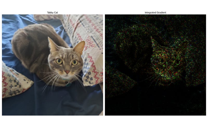
Now let's work on an image classification example, we will use resnet18 trained on ImageNet applied to a picture of my cat. We will use the exact same process as above and each image pixel will be considered as an input feature. We will get a result where each pixel is represented by how much it influenced the classification of the image as a Tabby cat.

We can see that pixels that mostly influenced the “Tabby Cat” output neuron are located on the face of the cat.

Conclusion:

Integrated Gradients is a great method to get some understanding of the influence of each input feature on the output of your neural network. This method solves some of the shortcomings of existing approaches and satisfies some axioms like Sensitivity and implementation invariance.
This approach can be a great tool when working on neural networks in order to better understand their predictions or even detect if there are some issues with the training algorithm or dataset.

Code: https://github.com/CVxTz/IntegratedGradientsPytorch