The application of machine learning techniques (such as linear regression) to classify a frequency filter from its spectrum
- Filter Classifier From Scratch
- Smoothening Algorithm
- Convolution Classifier (Cython)
- K-Means Clustering
- Generating Spectra For Testing
- Example Output
- Further Readings
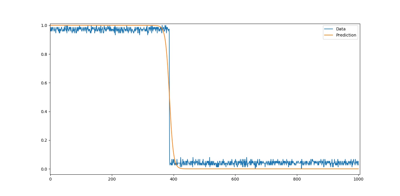
As opposed to the previous script (now called filterclassifierOLD.py) this one FilterClassifier.py can easily handle mildly noisy signals like those seen in the testspectra folder. Those signals were constructed by evaluating a logistic function with randomly generated parameters and then perturbed by a low-variance Gaussian noise. The optimisation is done using a gradient descent iterative algorithm (for each coefficient vector K, Kn+1 = Kn - ∇E dt where dt is the step size or "learning rate" or component-wise kn+1 = kn - ∂kE dt ) . The mean squared error was used as an error function E. The sum was used instead since the factor of 1/n is a constant and made irrelevant by the step size. Likewise for the factor of 2 in the partial derivatives so they were also omitted. I have also a more visual, Javascript version that I made which is available on the repository's page.
The method used can be considered to be a single-input perceptron model y = f(wx+b) where f is the activation function taken to be a logistic function f(x) = 1/1+exp(-wx-b). The following image is a good enough visual representation but the Y input is excluded

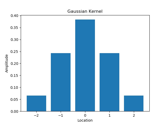
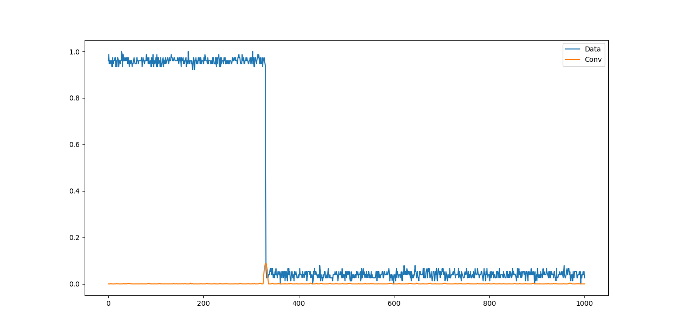
As a smoothening algorithm, the scriptSpectrumSmoothener.py draws inspiration from a blurring algorithm for images. It uses a normalised Gaussian kernel vector with components [7,26,41,26,7]. The Gaussian kernel was chosen in order to preserve most of the integrity of the individual data points while still providing sufficient weighting to remove the jaggedness. Other variations could be to use a Lorentzian (or a Cauchy for those outside of Physics) distribution to weight the blurring which is a thinner bell curve with thicker "tails" however for my purposes the Gaussian was sufficient. Something to keep in mind is that the more iterations performed, the less steep the cut-off gradient becomes so caution is to be taken when setting the iteration hyperparameter. Tests will be carried out on this in the future before being implemented in the main script to see whether it improves convergence and whether it skewes the results too far from the actual.
Documentation coming soon :)
There is merit to using K-means clustering in order to "compress" the data of the signal spectrum as seen in this sketch I created here. This can potentially be used both instead of smoothening and instead of the curve fitting due to how effective it is at reproducing the shape of the spectrum extremely fast. Also this could have the advantage of generalising further to band-pass filters and not just low/high-pass filters but that remains to be seen. I plan on making a more in-depth repository discussing K-means here.
The test spectra were generated by using an actual logistic function f(x) = A/1+exp((-1)n(mx-b)) where all the variables A, n, m, and b were selected at random for each spectrum. Some faint Gaussian noise with variable variance (that was also randomly selected) was then added to better emulate an actual reading. This can all be seen in the TestSpectra.py script.
A future addition that could be done to this is to randomly include sharp, delta-function dips or spikes in the spectra and see how well the model can navigate towards the solution with that big of an obstacle.
import spectrum number: 50
412.09381304786876
10.149479221295394
8.410639693560967
7.5498748688980895
7.001944267408166
...
3.4078254544385143
3.401236978917254
3.3947383786798913
3.388327526728673

w: -156.8231823034971  b: 60.583954796858976
Low-pass
Cut-off:  386.70646686847317
Step slope:  -39.205795575874276

Process finished with exit code 0
- https://delsquared.github.io/signal-frequency-filter-classifier/
- https://en.wikipedia.org/wiki/Gradient_descent
- https://en.wikipedia.org/wiki/Logistic_regression
- https://en.wikipedia.org/wiki/Regression_analysis
- https://en.wikipedia.org/wiki/Logistic_function
- https://en.wikipedia.org/wiki/Mathematical_optimization
- https://en.wikipedia.org/wiki/Perceptron
- https://en.wikipedia.org/wiki/K-means_clustering
- https://github.com/DelSquared/K-Means-Clustering-Visualisation
- https://delsquared.github.io/K-Means-Clustering-Visualisation