Actuarial Reserve Risk Classification with Gaussian Mixture

ARRC

Abstract : The loss triangle is effective in calculating the actuarial reserve. In this work, we will try to classify each number in this triangle into a specific category useful in estimating the risks associated with this. We will not focus too much on the loss triangle or use an innovative way to create it, but will focus more on making the classification creatively. The final shape of the loss triangle will be different, as it will be a heat map showing the different ratings for each number, Also we will use the new data generation from our model as a measure of the expectation of the missing part of the loss triangle.

You can easily download all the data file from Here and Here and Here and the last file is Here

start with this beautiful equation

where is the mean, the covariance matrix, and k is the dimension of the space where x takes values.

Here we will take much care of k which represents the number of mixes our data have . This can, of course, be seen with the naked eye by drawing the histogram like :

From above histogram it is clear that we are facing a mixture of two Gaussian distributions

Some problems with the data

Non common problems faced by many such as missing data and ... etc

Problem in the form of data when we draw histagram as we see here

Our data not really ideal for using the Gaussian model ! But the fun part is that it's like lognormal so we can convert it to normal or at least like normal using log transfrom

After applying log transform we have :

Here we see that the data is similar to the mixed Gaussian distribution with 2D note:The blue curves I put for illustration

As we thought, the EM algorithm decided that the distribution was 2D mixed

Let's start working with some codes:

# importing libs.

import pandas as pd
import seaborn as sns
from sklearn.mixture import GaussianMixture
from sklearn.model_selection import StratifiedKFold
from scipy.stats import multivariate_normal

# this our most important list 
groupby_list=['IncurredAgeBucket','CalYear','ClaimType','ClaimDuration','Gender']  

The idea is we will manipulate the classification of our target several times and make a set of models,this will make a set of loss triangles

We have big data and we don't know how to choose it in principle but we will loop it with fixed classifications that will be necessary to maintain chainladder rules.

#import data and use concat from pands to put all data file together
sorted_data=data.sort_values(['IncurredAgeBucket']).reset_index(drop=True) #sort and fix indixing

#This will help us to keep this class in our data 
#(Groupby function, excludes classifications if they are not inside the function, or deal with them in bad way)
groupby_=sorted_data.groupby([ groupby_list[0],groupby_list[1],groupby_list[2],
                              groupby_list[3],groupby_list[4]])
groupby_data=groupby_.sum().reset_index()
                                       #sum using groupby

Here we will replace the orignal name of this labels to make it more easy for us

by_data = pd.DataFrame(np.array(groupby_data))
groupby_data['IncurredAgeBucket'].replace(to_replace=['0-49'], value=int(0),inplace=True)
groupby_data['IncurredAgeBucket'].replace(to_replace=['50'], value=int(1),inplace=True)
groupby_data['IncurredAgeBucket'].replace(to_replace=['55'], value=int(2),inplace=True)
groupby_data['IncurredAgeBucket'].replace(to_replace=['60'], value=int(3),inplace=True)
groupby_data['IncurredAgeBucket'].replace(to_replace=['65'], value=int(4),inplace=True)
groupby_data['IncurredAgeBucket'].replace(to_replace=['70'], value=int(5),inplace=True)
groupby_data['IncurredAgeBucket'].replace(to_replace=['75'], value=int(6),inplace=True)
groupby_data['IncurredAgeBucket'].replace(to_replace=['80'], value=int(7),inplace=True)
groupby_data['IncurredAgeBucket'].replace(to_replace=['85'], value=int(8),inplace=True)
groupby_data['IncurredAgeBucket'].replace(to_replace=['90'], value=int(9),inplace=True)
groupby_data['IncurredAgeBucket'].replace(to_replace=['90+'], value=int(10),inplace=True)

groupby_data['Gender'].replace(to_replace=['M'], value=int(0),inplace=True)
groupby_data['Gender'].replace(to_replace=['F'], value=int(1),inplace=True)

groupby_data['ClaimType'].replace(to_replace=['ALF'], value=int(0),inplace=True)
groupby_data['ClaimType'].replace(to_replace=['HHC'], value=int(1),inplace=True)
groupby_data['ClaimType'].replace(to_replace=['NH'], value=int(2),inplace=True)
groupby_data['ClaimType'].replace(to_replace=['Unk'], value=int(3),inplace=True)

here we will use histogram to check our data shape

fig, ax = plt.subplots()
groupby_data['AmountPaid'].plot.kde(ax=ax, legend=False, title='Histogram: check normallaty ')
groupby_data['AmountPaid'].plot.hist(ax=ax)
y=stats.anderson(groupby_data['AmountPaid'], dist='norm') #sample estimates normallity test
if y[1][2] <0.05 :#check normality
    print('its follow normal')
elif y[1][2] > 0.05 :
    print('no its not normal')
#as we see above our data may(may not) follow normal distribution but it not in ideal shape, so we can do log transform 
#before using GP model 
#one reason that we decide to use log transform is that Histogram give us kind of lognormal shape

applying log transform and plot one more time

#In this code part and next code we will explain the way of ARRC work and dealing with G-mixtuer 
#So you can find the full documentation in the py file (You will find some part of this code inside big loop)
# Transform part using lN(x+1) if we use in future any predictive method we can reverse it using e^(x-1)
datatrans1=np.log1p(groupby_data['AmountPaid'])
new_=groupby_data[groupby_list[nu*2]].astype(np.int32) # nu here its the loop counter
datatrans=np.array([new_,datatrans1]).T # here we merge labels with data after log transform 


#check avelabilty to apply G-mixtuer model
fig, ax = plt.subplots()
pd.DataFrame(datatrans).plot.kde(ax=ax, legend=False, title='Histogram:check new shape for GP after log  ')
pd.DataFrame(datatrans).plot.hist(ax=ax)

Here we will start littel machine learning work we will break the data into two parts. The goal of this is to make one part test for the other.

# Break up the dataset into X train (75%) and X test (25%) sets.
skf = StratifiedKFold(n_splits=4)
# Only take the first fold.
train_index, test_index = next(iter(skf.split(datatrans,np.full(np.shape(datatrans)[0],1))))
#apply test and train to our data
X_train = datatrans[train_index]
X_test = datatrans[test_index]

As we know we are looking for target to class our data with supervise-learning the best job that our loop do for us is to test more than one label class that already in our data (you can see py file for more info)

let's code !

# here other intrsting part 
#find the best mixture number using bic with different covariances type
optimal=[]
for s in range (2,6):
    for cov_type in ['spherical', 'diag', 'tied', 'full'] :
            models=GaussianMixture(n_components=s, covariance_type=cov_type,max_iter=150,n_init=20
                                   ,random_state=500).fit(X_train)
            bic=models.bic(datatrans)# bic number
            optimal.append([bic,cov_type,s])

this is the equition of bic BIC = −2 lnL + k ln (n) wehre L is the maximized value of the likelihood function for the estimated model ,k is the number of free parameters , n number of observations Note that : you can here use AIC but since AIC dealing with small size sample and we have big sample size so i prefer to use BIC

We can plot this now to see the best mixture number for random sample

Remember : lowe bic is best

Regularization of the covariance matrix In many applications we may facing high dimensional problem , to avoide this problem we may use diffrant ways one of this way is that to add some value in the diagonal of matrix and this what we will do next

reg_=[0.0001,0.008,0.05,0.1,0.2,0.3,0.5]#useing different size to control covariance
for u in (reg_):
          estimators = {cov_type : GaussianMixture(n_components=n_classes,warm_start=True, # warm statrt to benefit from loop
                        covariance_type=cov_type, max_iter=300,n_init=20, reg_covar=u ,init_params=param,
                        random_state=np.random.randint(250,80000))
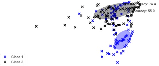
                        for cov_type in ['spherical', 'diag', 'tied', 'full']}

Here we will use mean as a measure of error and in our cases it's useful way because we develop our model benefit from labels that we have so in supervised manner its a good way to test accuracy

y_test_pred = estimator.predict(X_test)
test_accuracy = np.mean(y_test_pred.ravel() == y_test.ravel()) * 100

After we have finished modeling, and if we set a standard of accuracy, say, 70% or more,then we will prepare for the design of the loss triangle, and the same operations we do, will be simulated on our class [Class A , Class B ...etc]

loss_t_data=groupby_data #Data processing for loss triangle 
predi=estimator.predict(datatrans) # data after transformation (if data don't follow normal distribution)
loss_t_data['class']=predi #predict label for evry value that we have
pre_data = loss_t_data['AmountPaid'].groupby([loss_t_data['CalYear']
                                             ,loss_t_data['ClaimDuration']]).sum().reset_index()#sum our data with respect 

As we see above we summing AmountPaid respect to CalYear & ClaimDuration we make the same process for our label value

After the completion of the class prosses , we will have categorized the data in will have categorized the data in ClaimDuration inside CalYear Next step is sum prosses and the result will be for sure as percentage for each class

#sum our labels and convert it to percentage
creat_prob_for_class=[]
for o in range (12):
    for k in range (12):
        for i in range (n_classes):
            y=np.sum(np.array(class_for_Y_D[o][k])==i)/len(class_for_Y_D[o][k])
            creat_prob_for_class.append(y)

This is most important part of our model because it's an effective way of knowing the structure of risks, we'll explain this next

We've finished sum and have combined the labels into one list with our pre-processed data to become a loss triangle

Now we have labels, but the problem is how to figure out what each poster stands for (I mean for the risks).

So here we have to find a way to classify the classification into risk levels

suppouse that we have C=(c1,c2,c3...cn) and X=(x1,x2,...xn),where c is class corresponding to our observation and C list its not unique and x is observation then Cu=(c1,c2,c3) where Cu is unique class after apply sum in previous step we have here Cu , such that for every x we have unique Cu=(c1,c2,c3...ck) where k is the number of features or labels from model that we develop and ck < 1 .

Algorithm 1 : Find max(Cu) for all X then sum corresponding value of max(Cu) , Risk will be from the highest to smallest based on sum #this Algorithm I didn't use it

Algorithm 2 : Part one (Find Cu > 0.4 for all X) then Part 2 (sum corresponding value of Cu > 0.4) , Part 3(Risk will be from the highest to smallest based on sum) # this is the Algorithm that i use it

Algorithm 2 for classify the classification into risk levels

Risk_description_for_every_class=[]
for index_ in range (n_classes):
    ind_=np.where(np.array(pre_data)[:,index_+3]>.40)# Part one 
    le=len(ind_[0])
    x=sum(pre_data.iloc[ind_[0][[i for i in range(le)]]].iloc[:,2]) #Part 2 
    Risk_description_for_every_class.append([x,index_])
This_our_risk_class=sorted(Risk_description_for_every_class,reverse=True) # Part 3

The out put will be like

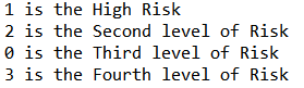
The semi-final out put is like :

As we see the colors show the level of risk accumulated within each number includes a set of insurance policies.

The final out put after triangle loss is :

---

---

We have finished, we now have a loss triangle and next to it a list containing the detail of each number in this triangle The detail will be the level of risk from which this number came because this number is the sum of the previous This will give the actuary the ability to know the level of risk it was in this year.

---

Support

Reach out to me by Email !

• Email onnoasd@hotmail.com

---