Reinforcement Learning with Model Predictive Control

Model Predictive Control-based Reinforcement Learning (mpcrl, for short) is a library for training model-based Reinforcement Learning (RL) [1] agents with Model Predictive Control (MPC) [2] as function approximation.

Documentation	https://mpc-reinforcement-learning.readthedocs.io/en/stable/
Download	https://pypi.python.org/pypi/mpcrl/
Source code	https://github.com/FilippoAiraldi/mpc-reinforcement-learning/
Report issues	https://github.com/FilippoAiraldi/mpc-reinforcement-learning/issues/

---

Introduction

This framework, also referred to as RL with/using MPC, was first proposed in [3] and has so far been shown effective in various applications, with different learning algorithms and more sound theory, e.g., [4, 5, 7, 8]. It merges two powerful control techinques into a single data-driven one

• MPC, a well-known control methodology that exploits a prediction model to predict the future behaviour of the environment and compute the optimal action

• and RL, a Machine Learning paradigm that showed many successes in recent years (with games such as chess, Go, etc.) and is highly adaptable to unknown and complex-to-model environments.

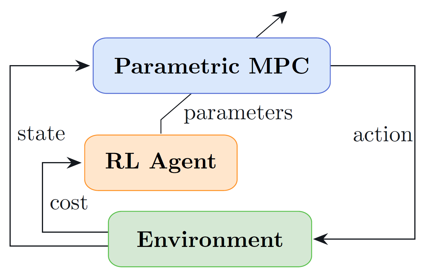
The figure below shows the main idea behind this learning-based control approach. The MPC controller, parametrized in its objective, predictive model and constraints (or a subset of these), acts both as policy provider (i.e., providing an action to the environment, given the current state) and as function approximation for the state and action value functions (i.e., predicting the expected return following the current control policy from the given state and state-action pair). Concurrently, an RL algorithm is employed to tune this parametrization of the MPC in such a way to increase the controller's performance and achieve an (sub)optimal policy. For this purpose, different algorithms can be employed, two of the most successful being Q-learning [4] and Deterministic Policy Gradient (DPG) [5].

---

Installation

Using pip

You can use pip to install mpcrl with the command

pip install mpcrl

mpcrl has the following dependencies

• Python 3.9 or higher
• csnlp
• SciPy
• Gymnasium
• Numba
• typing_extensions (only for Python 3.9)

If you'd like to play around with the source code instead, run

git clone https://github.com/FilippoAiraldi/mpc-reinforcement-learning.git

The main branch contains the main releases of the packages (and the occasional post release). The experimental branch is reserved for the implementation and test of new features and hosts the release candidates. You can then install the package to edit it as you wish as

pip install -e /path/to/mpc-reinforcement-learning

---

Getting started

Here we provide the skeleton of a simple application of the library. The aim of the code below is to let an MPC control strategy learn how to optimally control a simple Linear Time Invariant (LTI) system. The cost (i.e., the opposite of the reward) of controlling this system in state $s \in \mathbb{R}^{n_s}$ with action $a \in \mathbb{R}^{n_a}$ is given by

$$ L(s,a) = s^\top Q s + a^\top R a, $$

where $Q \in \mathbb{R}^{n_s \times n_s}$ and $R \in \mathbb{R}^{n_a \times n_a}$ are suitable positive definite matrices. This is a very well-known problem in optimal control theory. However, here, in the context of RL, these matrices are not known, and we can only observe realizations of the cost for each state-action pair our controller visits. The underlying system dynamics are described by the usual state-space model

$$ s_{k+1} = A s_k + B a_k, $$

whose matrices $A \in \mathbb{R}^{n_s \times n_s}$ and $B \in \mathbb{R}^{n_s \times n_a}$ could again in general be unknown. The control action $a_k$ is assumed bounded in the interval $[-1,1]$. In what follows we will go through the usual steps in setting up and solving such a task.

Environment

The first ingredient to implement is the LTI system in the form of a gymnasium.Env class. Fill free to fill in the missing parts based on your needs. The gymnasium.Env.reset method should initialize the state of the system, while the gymnasium.Env.steo method should update the state of the system based on the action provided and mainly return the new state and the cost.

from gymnasium import Env
from gymnasium.wrappers import TimeLimit
import numpy as np


class LtiSystem(Env):
    ns = ...  # number of states (must be continuous)
    na = ...  # number of actions (must be continuous)
    A = ...  # state-space matrix A
    B = ...  # state-space matrix B
    Q = ...  # state-cost matrix Q
    R = ...  # action-cost matrix R
    action_space = Box(-1.0, 1.0, (na,), np.float64)  # action space

    def reset(self, *, seed=None, options=None):
        super().reset(seed=seed, options=options)
        self.s = ...  # set initial state
        return self.s, {}

    def step(self, action):
        a = np.reshape(action, self.action_space.shape)
        assert self.action_space.contains(a)
        c = self.s.T @ self.Q @ self.s + a.T @ self.R @ a
        self.s = self.A @ self.s + self.B @ a
        return self.s, c, False, False, {}


# lastly, instantiate the environment with a wrapper to ensure the simulation finishes
env = TimeLimit(LtiSystem(), max_steps=5000)

Controller

As aforementioned, we'd like to control this system via an MPC controller. Therefore, the next step is to craft one. To do so, we leverage the csnlp package, in particular its csnlp.wrappers.Mpc class (on top of that, under the hood, we exploit this package also to compute the sensitivities of the MPC controller w.r.t. its parametrization, which are crucial in calculating the RL updates). In mathematical terms, the MPC looks like this:

$$ \begin{aligned} \min_{x_{0:N}, u_{0:N-1}} \quad & \sum_{i=0}^{N-1}{ x_i^\top \tilde{Q} x_i + u_i^\top \tilde{R} u_i } & \\ \textrm{s.t.} \quad & x_0 = s_k \\ & x_{i+1} = \tilde{A} x_i + \tilde{B} u_i, \quad & i=0,\dots,N-1 \\ & -1 \le u_k \le 1, \quad & i=0,\dots,N-1 \end{aligned} $$

where $\tilde{Q}, \tilde{R}, \tilde{A}, \tilde{B}$ do not necessarily have to match the environment's $Q, R, A, B$ as they represent a possibly approximated a priori knowledge on the sytem. In code, we can implement this as follows.

import casadi as cs
from csnlp import Nlp
from csnlp.wrappers import Mpc

N = ...  # prediction horizon
mpc = Mpc[cs.SX](Nlp(), N)

# create the parametrization of the controller
nx, nu = LtiSystem.ns, LtiSystem.na
Atilde = mpc.parameter("Atilde", (nx, nx))
Btilde = mpc.parameter("Btilde", (nx, nu))
Qtilde = mpc.parameter("Qtilde", (nx, nx))
Rtilde = mpc.parameter("Rtilde", (nu, nu))

# create the variables of the controller
x, _ = mpc.state("x", nx)
u, _ = mpc.action("u", nu, lb=-1.0, ub=1.0)

# set the dynamics
mpc.set_dynamics(lambda x, u: Atilde @ x + Btilde @ u, n_in=2, n_out=1)

# set the objective
mpc.minimize(
    sum(cs.bilin(Qtilde, x[:, i]) + cs.bilin(Rtilde, u[:, i]) for i in range(N))
)

# initiliaze the solver with some options
opts = {
    "print_time": False,
    "bound_consistency": True,
    "calc_lam_x": True,
    "calc_lam_p": False,
    "ipopt": {"max_iter": 500, "sb": "yes", "print_level": 0},
}
mpc.init_solver(opts, solver="ipopt")

Learning

The last step is to train the controller using an RL algorithm. For instance, here we use Q-Learning. The idea is to let the controller interact with the environment, observe the cost, and update the MPC parameters accordingly. This can be achieved by computing the temporal difference error

$$ \delta_k = L(s_k, a_k) + \gamma V_\theta(s_{k+1}) - Q_\theta(s_k, a_k), $$

where $\gamma$ is the discount factor, and $V_\theta$ and $Q_\theta$ are the state and state-action value functions, both provided by the parametrized MPC controller with $\theta = {\tilde{A}, \tilde{B}, \tilde{Q}, \tilde{R}}$. The update rule for the parameters is then given by

$$ \theta \gets \theta + \alpha \delta_k \nabla_\theta Q_\theta(s_k, a_k), $$

where $\alpha$ is the learning rate, and $\nabla_\theta Q_\theta(s_k, a_k)$ is the sensitivity of the state-action value function w.r.t. the parameters. All of this can be implemented as follows.

from mpcrl import LearnableParameter, LearnableParametersDict, LstdQLearningAgent
from mpcrl.optim import GradientDescent

# give some initial values to the learnable parameters (shapes must match!)
learnable_pars_init = {"Atilde": ..., "Btilde": ..., "Qtilde": ..., "Rtilde": ...}

# create the set of parameters that should be learnt
learnable_pars = LearnableParametersDict[cs.SX](
    (
        LearnableParameter(name, val.shape, val, sym=mpc.parameters[name])
        for name, val in learnable_pars_init.items()
    )
)

# instantiate the learning agent
agent =  LstdQLearningAgent(
    mpc=mpc,
    learnable_parameters=learnable_pars,
    discount_factor=...,  # a number in (0,1], e.g.,  1.0
    update_strategy=...,  # an integer, e.g., 1
    optimizer=GradientDescent(learning_rate=...),
    record_td_errors=True,
)

# finally, launch the training for 5000 timesteps. The method will return an array of
# (hopefully) decreasing costs
costs = agent.train(env=env, episodes=1, seed=69)

---

Examples

Our examples subdirectory contains examples on how to use the library on some academic, small-scale application (a small linear time-invariant (LTI) system), tackled both with on-policy Q-learning, off-policy Q-learning and DPG. While the aforementioned algorithms are all gradient-based, we also provide an example on how to use Bayesian Optimization (BO) [6] to tune the MPC parameters in a gradient-free way.

---

License

The repository is provided under the MIT License. See the LICENSE file included with this repository.

---

Author

Filippo Airaldi, PhD Candidate [f.airaldi@tudelft.nl | filippoairaldi@gmail.com]

Delft Center for Systems and Control in Delft University of Technology

Copyright (c) 2024 Filippo Airaldi.

Copyright notice: Technische Universiteit Delft hereby disclaims all copyright interest in the program “mpcrl” (Reinforcement Learning with Model Predictive Control) written by the Author(s). Prof. Dr. Ir. Fred van Keulen, Dean of ME.

---

References

[1] Sutton, R.S. and Barto, A.G. (2018). Reinforcement learning: An introduction. Cambridge, MIT press.

[2] Rawlings, J.B., Mayne, D.Q. and Diehl, M. (2017). Model Predictive Control: theory, computation, and design (Vol. 2). Madison, WI: Nob Hill Publishing.

[3] Gros, S. and Zanon, M. (2020). Data-Driven Economic NMPC Using Reinforcement Learning. IEEE Transactions on Automatic Control, 65(2), 636-648.

[4] Esfahani, H. N. and Kordabad, A. B. and Gros, S. (2021). Approximate Robust NMPC using Reinforcement Learning. European Control Conference (ECC), 132-137.

[5] Cai, W. and Kordabad, A. B. and Esfahani, H. N. and Lekkas, A. M. and Gros, S. (2021). MPC-based Reinforcement Learning for a Simplified Freight Mission of Autonomous Surface Vehicles. 60th IEEE Conference on Decision and Control (CDC), 2990-2995.

[6] Garnett, R., 2023. Bayesian Optimization. Cambridge University Press.

[7] Gros, S. and Zanon, M. (2022). Learning for MPC with stability & safety guarantees. Automatica, 164, 110598.

[8] Zanon, M. and Gros, S. (2021). Safe Reinforcement Learning Using Robust MPC. IEEE Transactions on Automatic Control, 66(8), 3638-3652.