This script looks to account for spatial autocorrelation in spatial regression modeling through various methods, including trend surface modeling and eigenvector mapping!
# Read in Thrush Presence/Absence Point Data
point.data <- read.csv(here::here("Data", "vath_2004.csv"), header=TRUE)

# Read in Elevation DEM
elev = raster(here::here("Data", "elev.gri"))We want to create a spatial regression by utilizing terrain features such as elevation & slope to infer Thrush locations.
# 1. Create slope, aspect layers from elevation
elev.terr <- terrain(elev, opt=c("slope", "aspect"))

# 2. Prepare Layers for Extraction
layers        <- stack(elev, elev.terr)
names(layers) <- c("elev", "slope", "aspect")

# 3. Extract GIS data at sampling points
coords   <- cbind(point.data$EASTING, point.data$NORTHING)
land.cov <- extract(x=layers, y=coords)

# 4. Append Spatial Data to Thrush Dataset
point.data <- cbind(point.data,land.cov)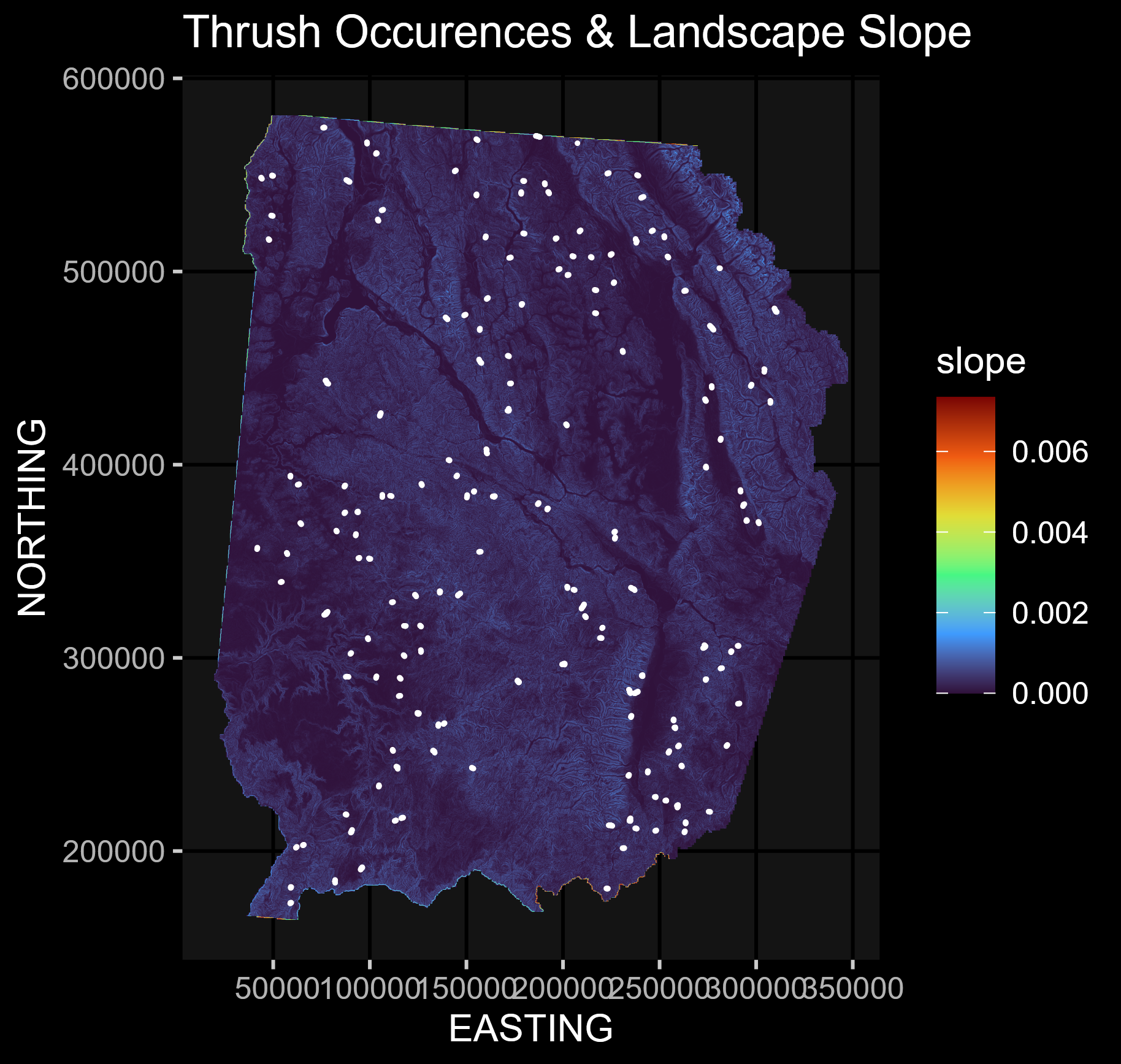
To do a Polynomial Trend Surface Model, you want to add the linear, quadratic, and cubic terms--which you can do manually or with poly(). poly(EASTING,3) and poly(NORTHING,3) would add the linear, quadratic and cubic terms instead of adding them all yourself. Note that the poly function also standardizes polynomials to be orthogonal, removing the correlation between terms (which in many situations would be preferred).
# 1. Create a Polynomial Trend Surface Model
VATH.trend <- glm(VATH~elev+I(elev^2)+EASTING+NORTHING+I(EASTING^2)+
                    I(EASTING^3)+I(NORTHING^2)+I(NORTHING^3), family="binomial", data=point.data)
# Note: This is equivalent to
VATH.trend <- glm(VATH~elev+I(elev^2)+poly(EASTING,3)+poly(NORTHING,3), family="binomial", data=point.data)

# 2. Extract Model Coefficients
trend.summary <- c(summary(VATH.trend)$coef[2,1],
                   summary(VATH.trend)$coef[2,2],
                   summary(VATH.trend)$coef[3,1],
                   summary(VATH.trend)$coef[3,2])

# 3. Extract Model Residuals
VATH.trend.res <- residuals(VATH.trend, type="deviance")

# 4. Create Indicator Correlogram on Residuals of the Polynomial Trend Surface Model
cor.trend.res <- icorrelogram(locations=coords, z=VATH.trend.res, binsize=1000, maxdist=15000)

# 5. Plot Residual Indicator Correlogram
plot(cor.trend.res$dist, cor.trend.res$Morans.i, ylim = c(-0.5, 0.5), main = "Polynomial Trend Surface Residual Correlogram")
abline(h=0, lty = "dashed")
lines(cor.trend.res$dist, cor.trend.res$null.lcl)
lines(cor.trend.res$dist, cor.trend.res$null.ucl)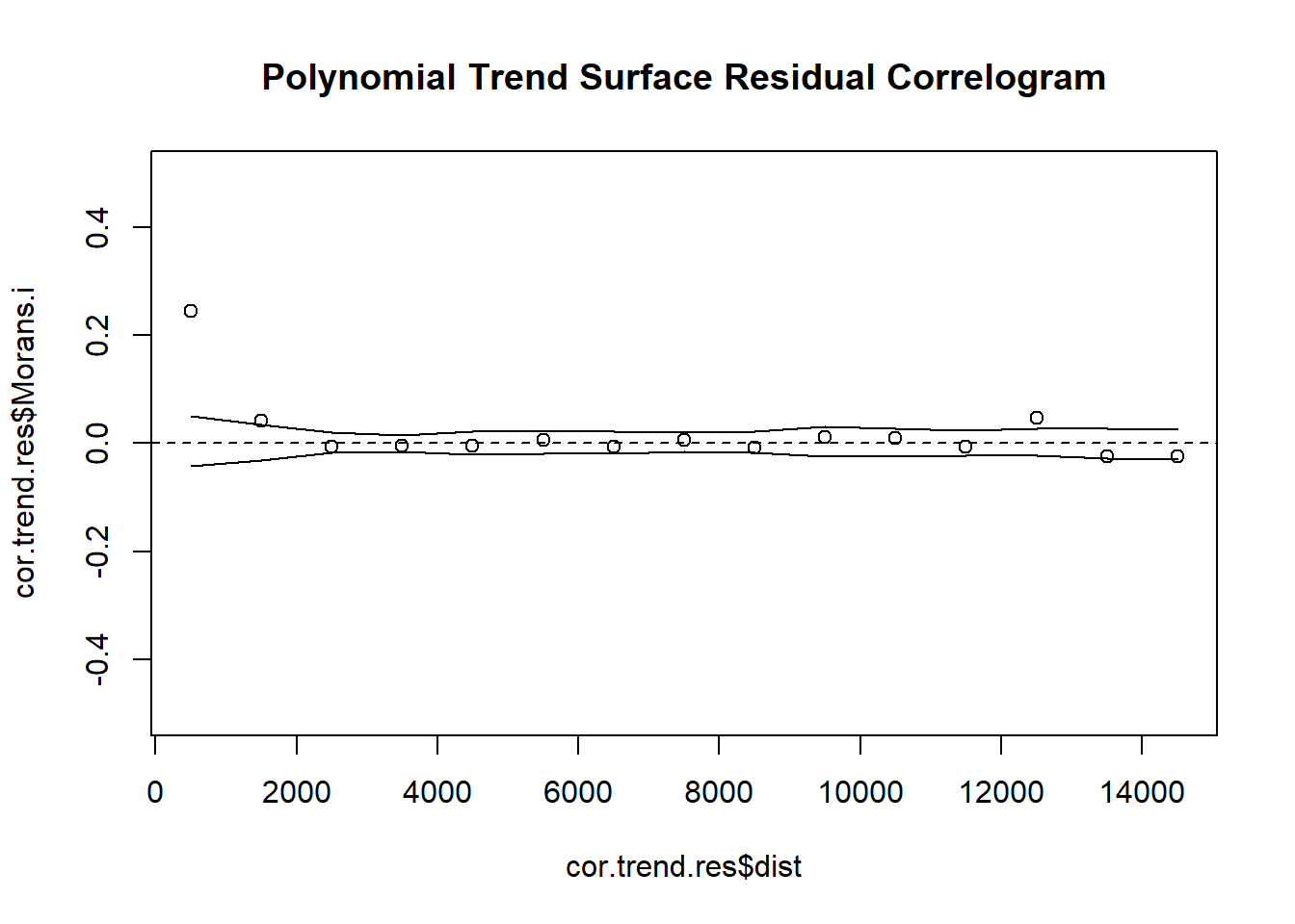
The Polynomial Trend Surface Model is limited in the spatial variation in can capture. An alternative to this model is to consider a generalized additive model (GAM), where we allow spline functions to capture spatial variation. The mgcv package provides a means to automate the selection of spline variation through the use of generalized cross-validation procedures Splines are considered for both Easting (x) and Northing ( y) coordinates with the s() command! *This syntax defaults to automated selection of the number of knots being considered
# 1. Generate GAM Trend Surface Model
VATH.gam <- gam(VATH~elev+I(elev^2)+s(EASTING,NORTHING), family="binomial", data=point.data)

# 2. Inspect the Model
summary(VATH.gam)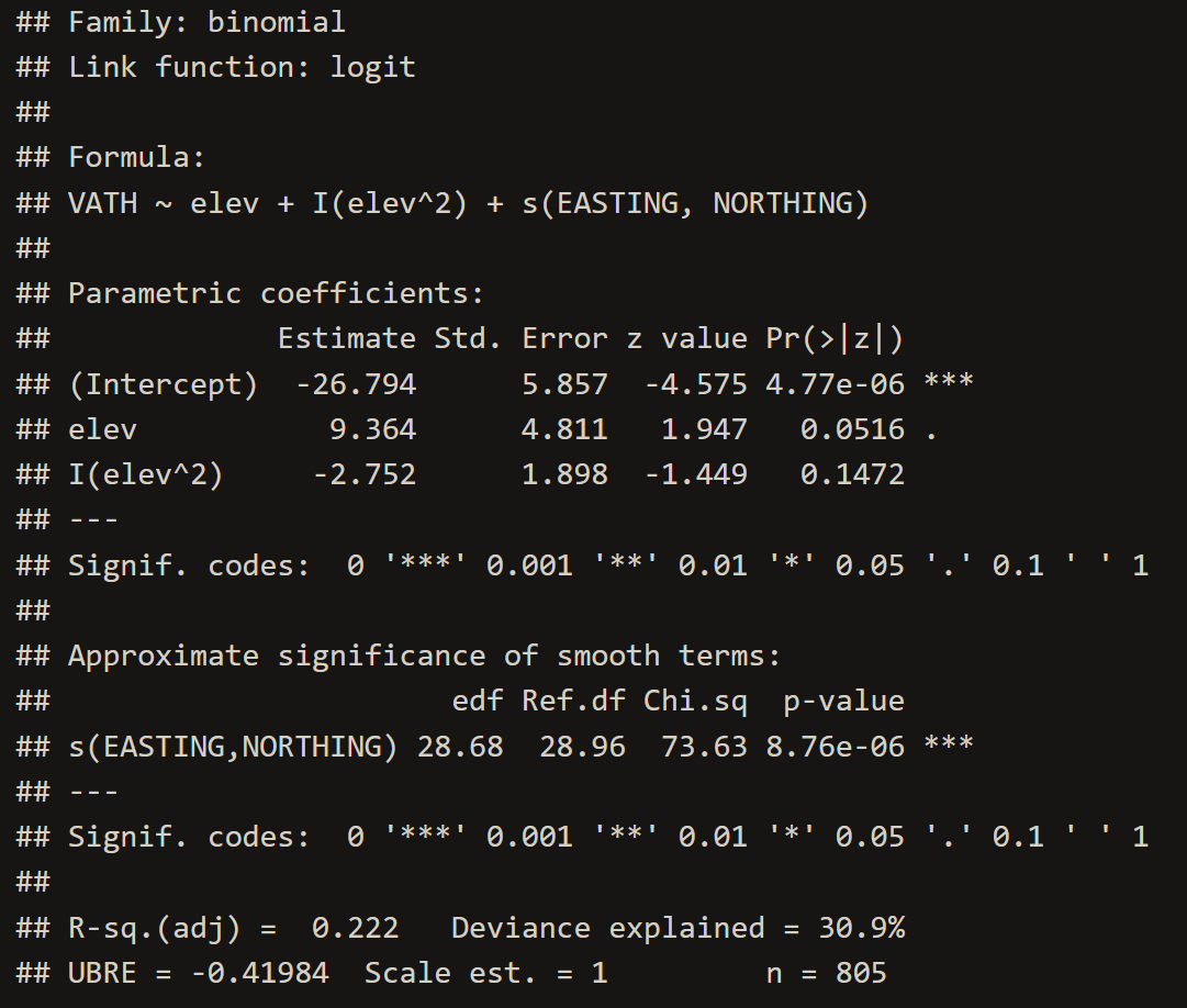
# 3. Extract Model Coefficients
gam.summary <- c(summary(VATH.gam)$p.coeff[2],
                 summary(VATH.gam)$se[2],
                 summary(VATH.gam)$p.coeff[3],
                 summary(VATH.gam)$se[3])

# 4. Extract Model Residuals
VATH.gam.res <- residuals(VATH.gam, type="deviance")

# 5. Create Indicator Correlogram on Residuals of the GAM Trend Surface Model
cor.gam.res <- icorrelogram(locations=coords, z=VATH.gam.res, binsize=1000, maxdist=15000)

# 6. Plot Residual Indicator Correlogram
plot(cor.gam.res$dist, cor.gam.res$Morans.i, ylim = c(-0.5, 0.5), main = "GAM Residual Correlogram")
abline(h=0, lty = "dashed")
lines(cor.gam.res$dist, cor.gam.res$null.lcl)
lines(cor.gam.res$dist, cor.gam.res$null.ucl)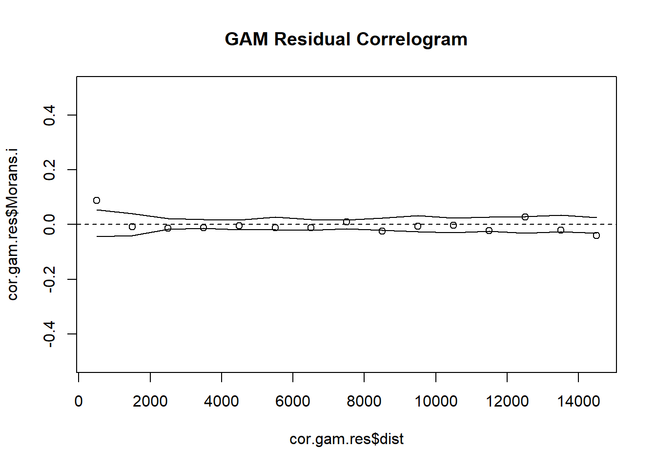
Moran Eigenvector (ME) is intended to remove spatial autocorrelation from the residuals of generalised linear models. We can use this to remove autocorelated points in our Thrush data!
We want to calculate a neighborhood weights matrix by using the maximum distance needed for a minimum spanning tree—the minimum set of connections needed to fully connect points across the landscape. The distance needed for a minimum spanning tree can be determined with the vegan package using the spantree function. Note that this distance could also be determined using the pcnm function and finding the threshold
# 1. Determine Threshold Distance Based on Minimum Spanning Tree
spantree.em <- spantree(dist(coords), toolong = 0)
max(spantree.em$dist)

# 2. Create a Neighbhorhood Matrix
dnn<- dnearneigh(coords, 0, max(spantree.em$dist))                   # List of links to neighboring points within distance range
dnn_dists <- nbdists(dnn, coords)                                    # List of distances (based on links in dnn)
dnn_sims <- lapply(dnn_dists, function(x) (1-((x/4)^2)))             # Scale distances as recommended by Dormann et al. (2007)
ME.weight <- nb2listw(dnn, glist=dnn_sims, style="B", zero.policy=T) # Create spatial weights matrix (in list form)

# 3. Determine Eigenvector Model Selection
VATH.ME <- spatialreg::ME(VATH~elev+I(elev^2), listw=ME.weight, family="binomial", data=point.data)# 1. Create New GLM with Eigenvector Adjusted Covariates
VATH.evm <- glm(VATH~elev+I(elev^2)+fitted(VATH.ME), family="binomial", data=point.data)
# 2. Inspect Eigenvector GLM Model
summary(VATH.evm)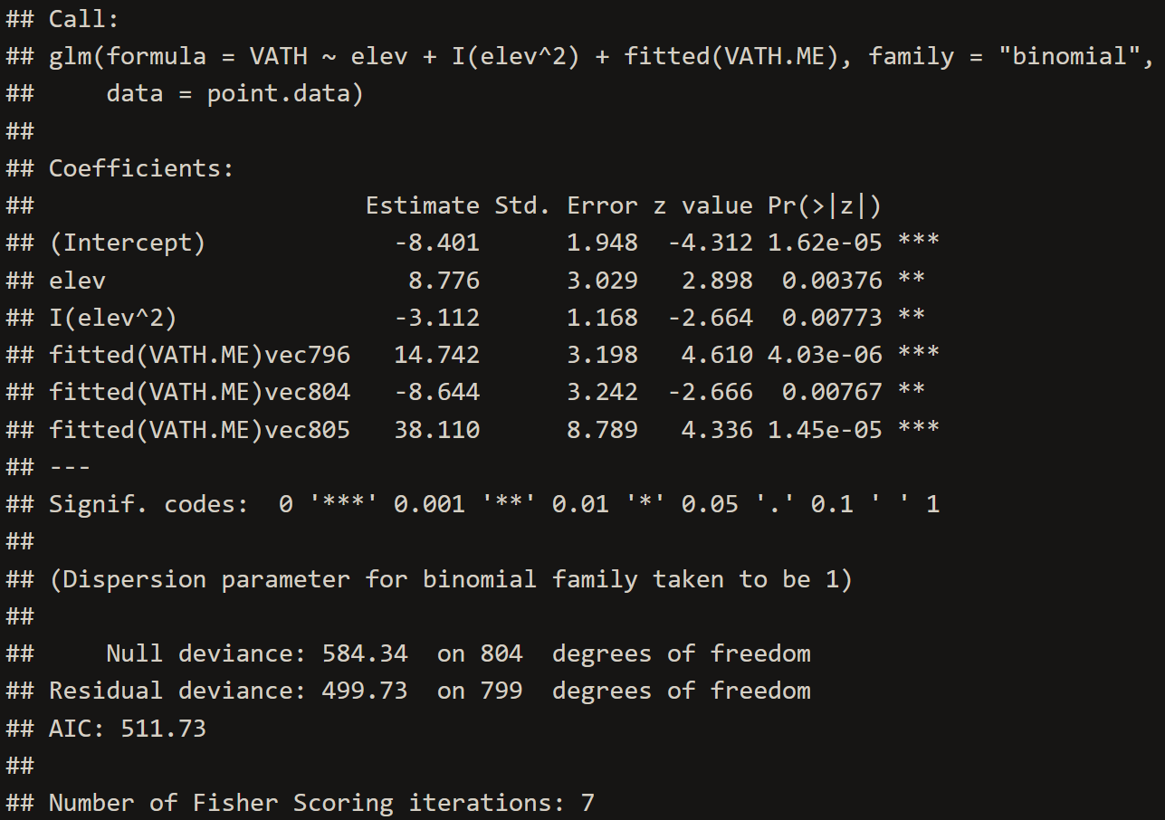
# 3. Extract coefficients
evm.summary <- c(summary(VATH.evm)$coef[2,1],
                 summary(VATH.evm)$coef[2,2],
                 summary(VATH.evm)$coef[3,1],
                 summary(VATH.evm)$coef[3,2])

# 4. Extract Model Residuals
VATH.evm.res <- residuals(VATH.evm, type="deviance")

# 5. Create Indicator Correlogram on Residuals of the Eigenvector GLM Model
cor.evm.res <- icorrelogram(locations=coords, z=VATH.evm.res, binsize=1000, maxdist=15000)

# 6. Plot Residual Indicator Correlogram
plot(cor.evm.res$dist, cor.evm.res$Morans.i, ylim = c(-0.5, 0.5), main = "Eigenvector Residual Correlogram")
abline(h=0, lty = "dashed")
lines(cor.evm.res$dist, cor.evm.res$null.lcl)
lines(cor.evm.res$dist, cor.evm.res$null.ucl)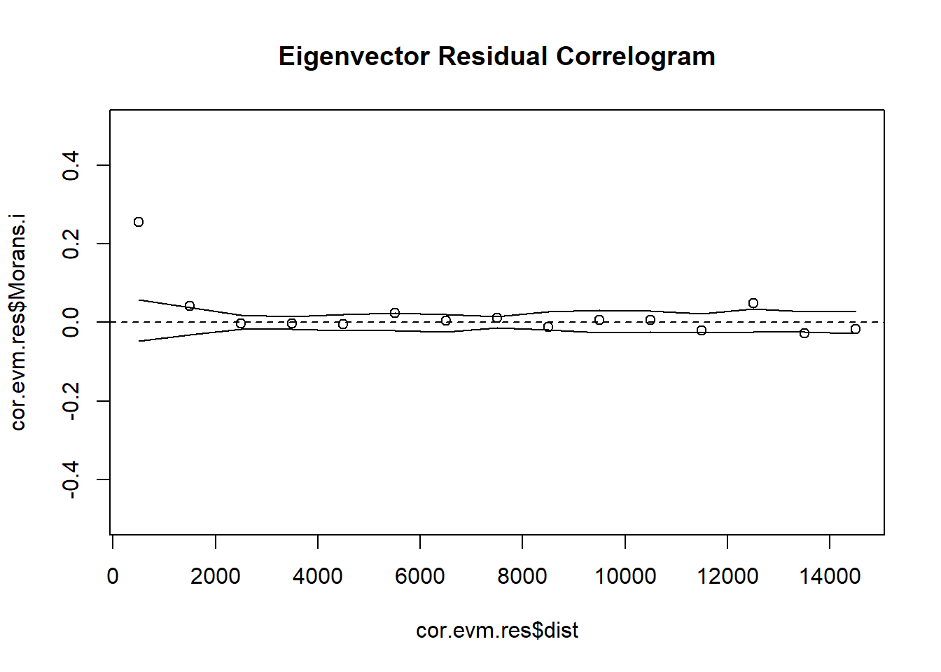
# 7. Plot Eigenvectors & Predicted Map
plot(glm.raster, xlab = "Longitude", ylab = "Latitude")
points(point.data[,c("EASTING","NORTHING")], pch=21, col="black", cex=2,lwd = 0.5,
bg=topo.colors(6)[cut(fitted(VATH.ME)[,1],breaks = 6)])To fit autocovariate models, we calculate new autocovariates and then use these covariates in a standard logistic regression model.
The type provides the weighting scheme.
-
When inverse is specified, points are weighted by the inverse of the distance between the focal point and the neighboring point.
-
When “one” is specified, all points within the distance (nbs) are given equal weight.
The style describes how the covariate will be calculated
- "B" reflects a binary coding, which provides a valid weighting scheme for autocovariate models!
# 1. Create Alternative Autocovariates with 1km radius
auto1km_inv <- autocov_dist(point.data$VATH, coords, nbs = 1000, type= "inverse",       # Inverse of distance weights
                            zero.policy=T)
auto1km     <- autocov_dist(point.data$VATH, coords, nbs = 1000, type= "one",style="B", # Binary weights
                            zero.policy=T)

# 2. Contrast Autocovariates with 1km radius
cor(auto1km, auto1km_inv)

# 3. Plot Autocovariates
par(mfrow = c(1,2))
plot(auto1km, auto1km_inv)
plot(jitter(auto1km, factor=0.4), auto1km_inv) # x-axis jittered to better see points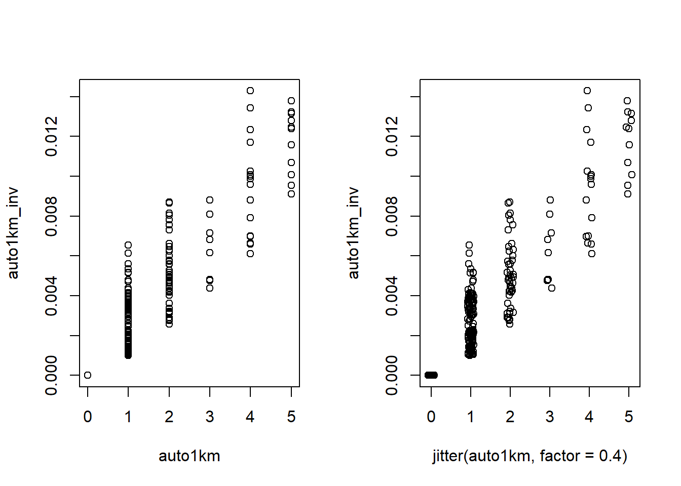
# 4. Create an Autocovariate Model
VATH.auto1km <- glm(VATH~elev+I(elev^2)+auto1km, family="binomial", data=point.data)

# 5. Inspect Autocovariate Model
summary(VATH.auto1km)

# 6. Extract Model Coefficients
auto.summary <- c(summary(VATH.auto1km)$coef[2,1],
                  summary(VATH.auto1km)$coef[2,2],
                  summary(VATH.auto1km)$coef[3,1],
                  summary(VATH.auto1km)$coef[3,2])

# 7. Extract Model Residuals
VATH.auto.res <- residuals(VATH.auto1km, type="deviance")

# 8. Create Indicator Correlogram on Residuals of the Autocovariate Model
cor.auto.res <- icorrelogram(locations=coords, z=VATH.auto.res, binsize=1000, maxdist=15000)

# 9. Plot Residual Indicator Correlogram
plot(cor.auto.res$dist, cor.auto.res$Morans.i, ylim = c(-0.5, 0.5), main = "Autocovariate Logistic Regressive Model Residual Correlogram")
abline(h=0, lty = "dashed")
lines(cor.auto.res$dist, cor.auto.res$null.lcl)
lines(cor.auto.res$dist, cor.auto.res$null.ucl)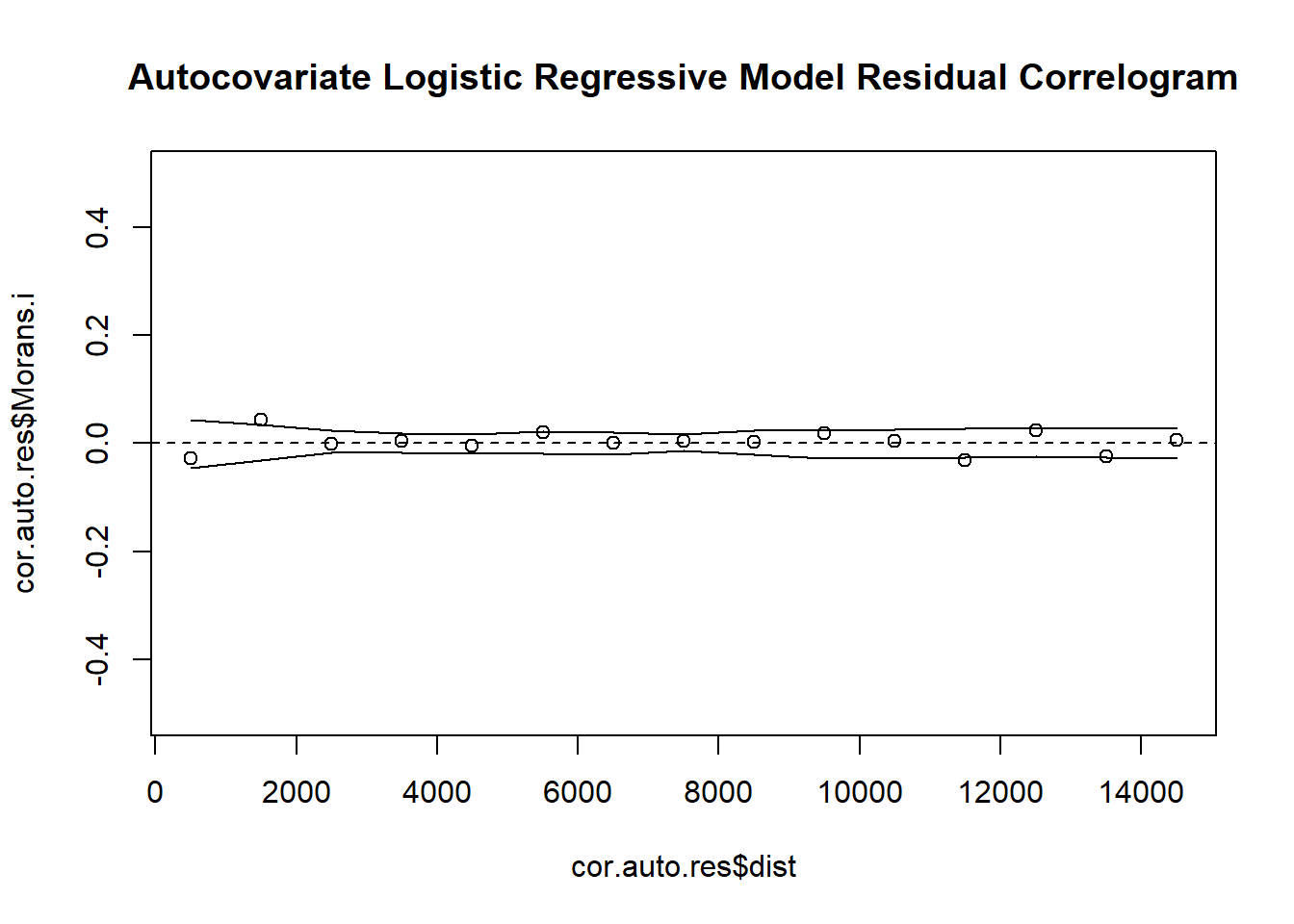
A simple multilevel model can also be fit to these data by considering transects as a random effect in the regression model. In doing so, we effectively “block” with transects, treating points within transects has having potential spatial dependence. Because this structure is not spatially explicit, we effectively assume that dependence is constant within transects (e.g., neighboring points have the same dependence as points located along the ends of the transects).
# 1. Ensure Random Effects are Factors
point.data$TRANSECT <- as.factor(point.data$TRANSECT)

# 2. Create a GLMM
VATH.glmm <- glmer(VATH~elev+I(elev^2)+(1|TRANSECT), family="binomial", data=point.data)

# 3. Inspect the GLMM
summary(VATH.glmm)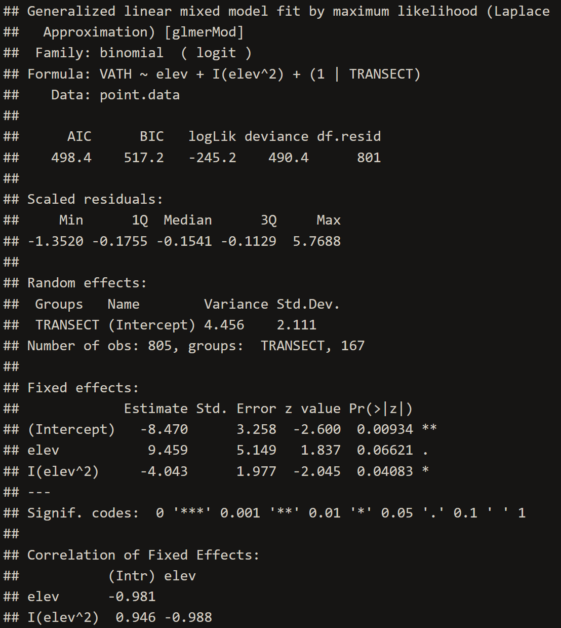
# 4. Extract Model Coefficients
glmm.summary <- c(summary(VATH.glmm)$coef[2,1],
                  summary(VATH.glmm)$coef[2,2],
                  summary(VATH.glmm)$coef[3,1],
                  summary(VATH.glmm)$coef[3,2])
# 5. Extract Model Residuals
VATH.glmm.res <- resid(VATH.glmm)

# 6. Create Indicator Correlogram on Residuals of the GLMM
cor.glmm.res <- icorrelogram(locations=coords, z=VATH.glmm.res, binsize=1000, maxdist=15000)

# 7. Plot Residual Indicator Correlogram
plot(cor.glmm.res$dist, cor.glmm.res$Morans.i, ylim = c(-0.5, 0.5), main = "Multilevel Model Residual Correlogram")
abline(h=0, lty = "dashed")
lines(cor.glmm.res$dist, cor.glmm.res$null.lcl)
lines(cor.glmm.res$dist, cor.glmm.res$null.ucl)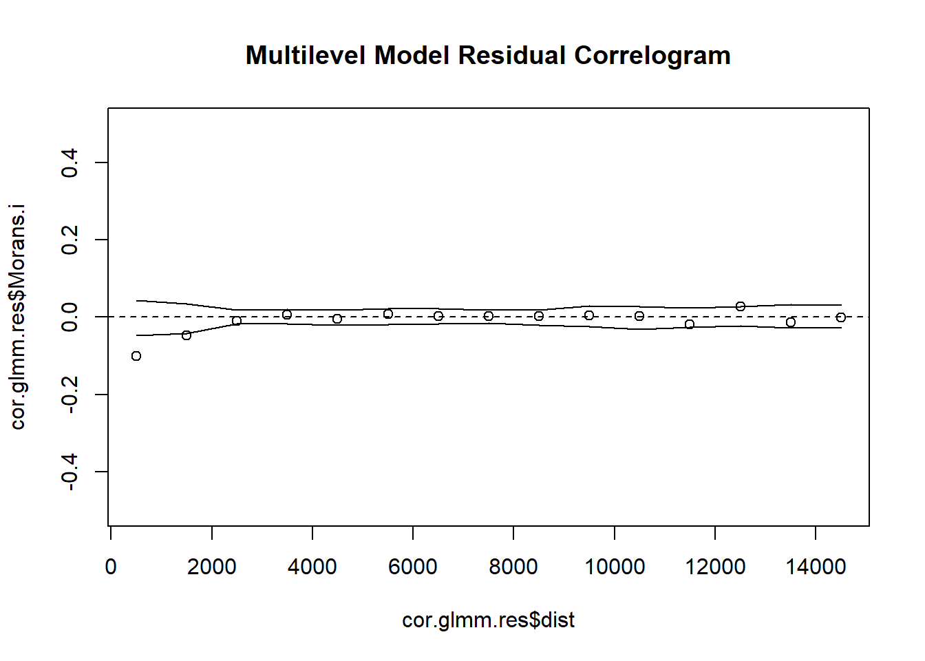
rmse = function(fit) return (sqrt(mean(residuals(fit)^2)))
fits_rmse = data.frame(
  model = c("Logistic Regression Ignoring Spatial Dependence",
            "Substituted Logistic Regression Ignoring Spatial Dependence",
            "Polynomial Trend Surface Model",
            "GAM Trend Surface Model",
            "Eigenvector Model",
            "Autocovariate Logistic Regression",
            "Multi-level Model"),
  rmse = c(
    rmse(VATH.elev2),
    rmse(VATH.sub),
    rmse(VATH.trend),
    rmse(VATH.gam),
    rmse(VATH.evm),
    rmse(VATH.auto1km),
    rmse(VATH.glmm)
  ))
fits_rmse
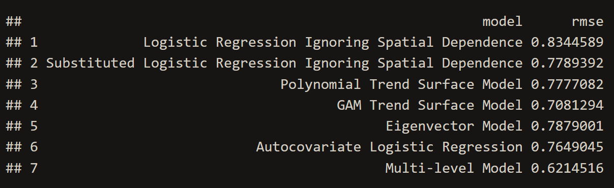
The lower the RMSE, the better a given model is able to fit a dataset--meaning that the Multi-level and GAM Trend Surface Model are the best models to choose from. The GAM Trend Surface Model did not successfully remove spatial dependence in the residuals while the Multi-level model did. The Multi-level model is the obvious choice, sporting both a low RMSE value and a removal of spatial dependence in the residuals.
Autocovariate and multilevel models did remove spatial dependence in the residuals by appropriately capturing the spatial scale of dependence in the data.