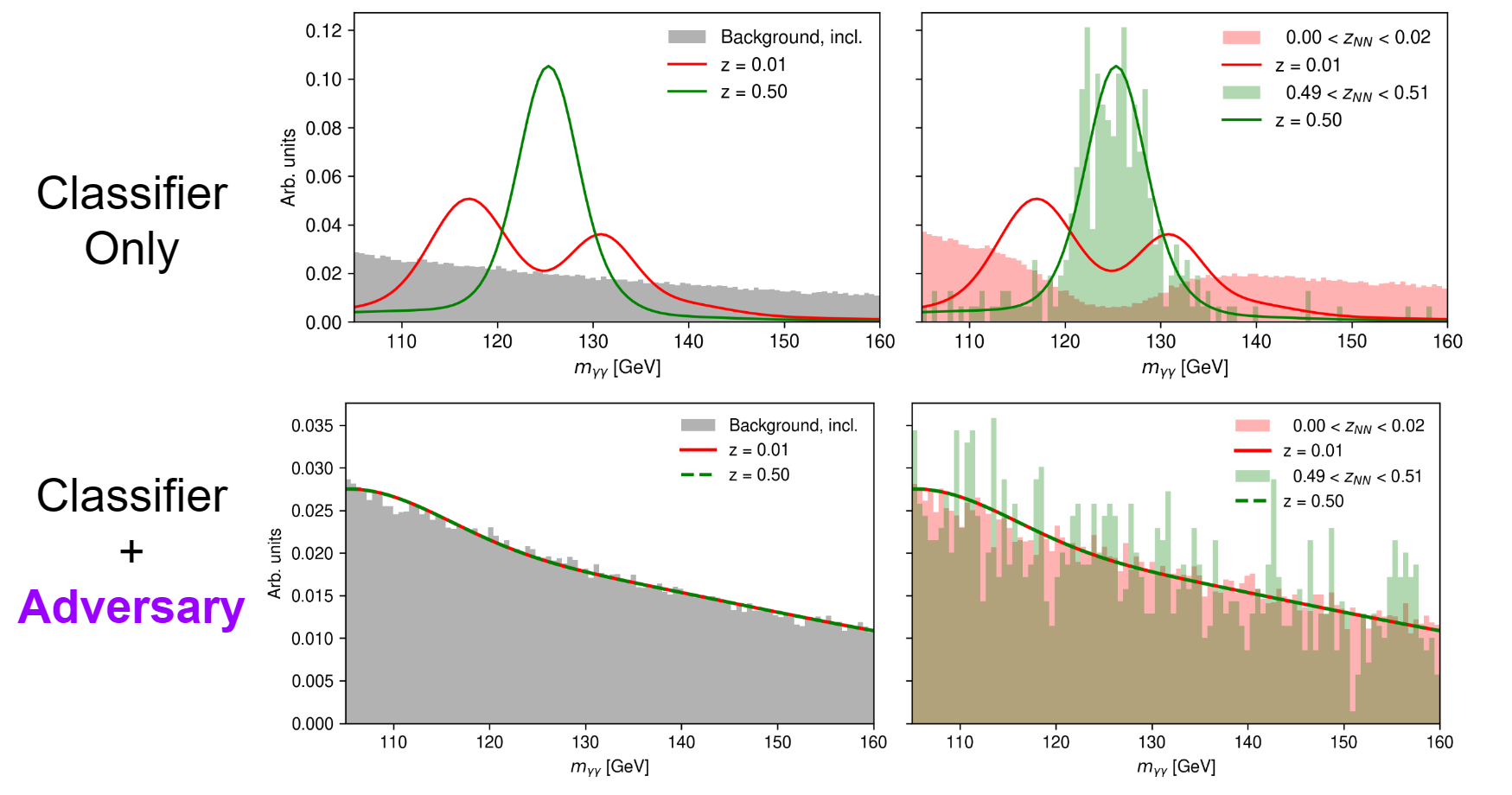
This study adapts the adversarial techniques introduced in "Decorrelated Jet Substructure Tagging using Adversarial Neural Networks" (https://arxiv.org/pdf/1703.03507) for applications in Higgs physics.
I addressed the problem of background mass sculpting in the Higgs to diphoton decay channel. This problem represents a biased selection of background events, where the background mass distribution is shaped to look like the signal mass distribution. This problem arises when a supervised classifier exploits correlations between training variables and the background mass.
ATLAS solves this problem by removing variables highly correlated with the diphoton invariant mass, detrimentally reducing the training data.
I tackled this problem by combining the classifier with an adversarial neural network (ANN). The ANN builds a Gaussian mixture model (GMM) to predict the background mass using the classifier’s score of true background events. The ANN’s loss is added to the classifier’s loss. During training, the classifier is penalised if the ANN can find correlations between the classifier’s background score and the mass. The classifier is prohibited from learning the correlations and can use the extra training variables discarded by ATLAS. My solution outperformed the state-of-the-art ATLAS classification, achieving 30% lower background efficiency for the same signal efficiency.
The plots on the right (above) show the background mass distributions for classifier scores (Z_NN) in the ranges 0-0.02 and 0.49-0.51. The Z_NN score signifies how much the classifier thinks a given event is a signal. In the classifier-only case, there is a clear sculpting in both mass ranges. For the adversary+classifier case, the distributions are identical between the two ranges, showing that background sculpting is successfully removed. To demonstrate the GMM fit, the adversary was trained at the end for both scenarios and the learned fit is displayed. The plots on the left overlay the GMM fits over the inclusive background distributions before any cuts are made to compare the distribution shapes before and after classification for both scenarios.
Overview presentation slides of this study can be found in MPhys overview slides.pdf.
First need the PowhegPy8EG_NNPDF30_VBFH125mc16a.csv (Higgs->diphoton signal) and Sherpa2_yyjj_njetGeq2_mjj_gt350.csv (non-resonant background) datasets.
Sequence to run the notebooks to generate the results:
- Generate ANN engineered features
- Combine ANN features
- ANN benchmark performance with 5% myy corr.
- ANN training (hyperparameter optimisation)
layers.py and ops.py are local import files used in notebooks 3 and 4.
Many thanks to my supervisor Dr. Liza Mijovic for her invaluable suggestions and advice during this study.
