Project by TomMakesThings - 2020/2021
𝗖𝗼𝗻𝘁𝗲𝗻𝘁𝘀
This respository hosts the datasets, code, interactive graphs and website for my undergraduate final year project. The aim is to experiment with clustering and topological data analysis to detect hidden gene expression in three different types of datasets. For an overview of the work, refer to this respository's GitHub Pages site, or read the PDF report here. If you'd like to experiment with the code yourself, refer to the Running the Code.
𝗖𝗹𝘂𝘀𝘁𝗲𝗿𝗶𝗻𝗴
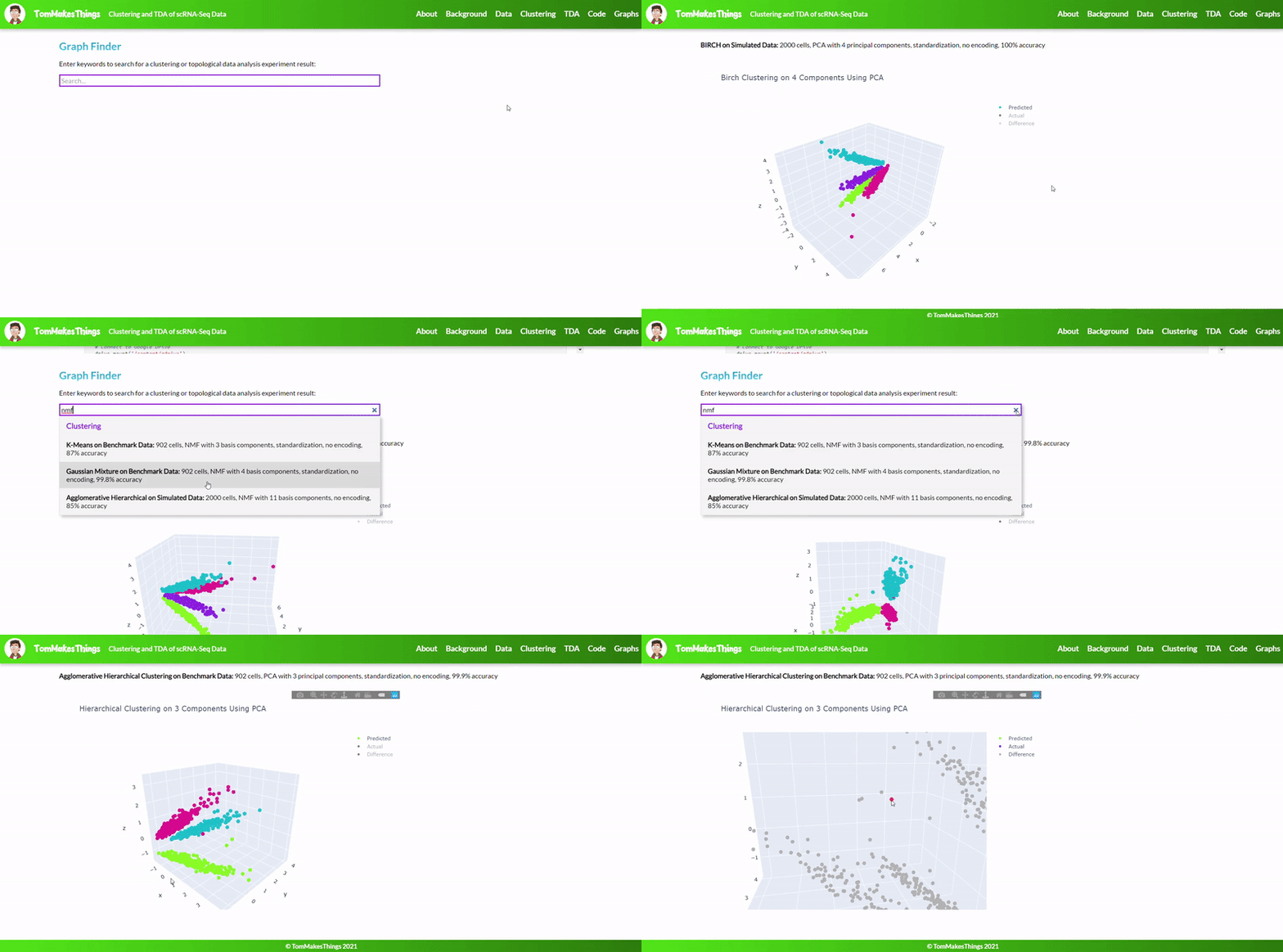
Different combinations of the pre-processing, dimensionality reduction methods and clustering algorithm were tested with the best combination varying per dataset.
Benchmark
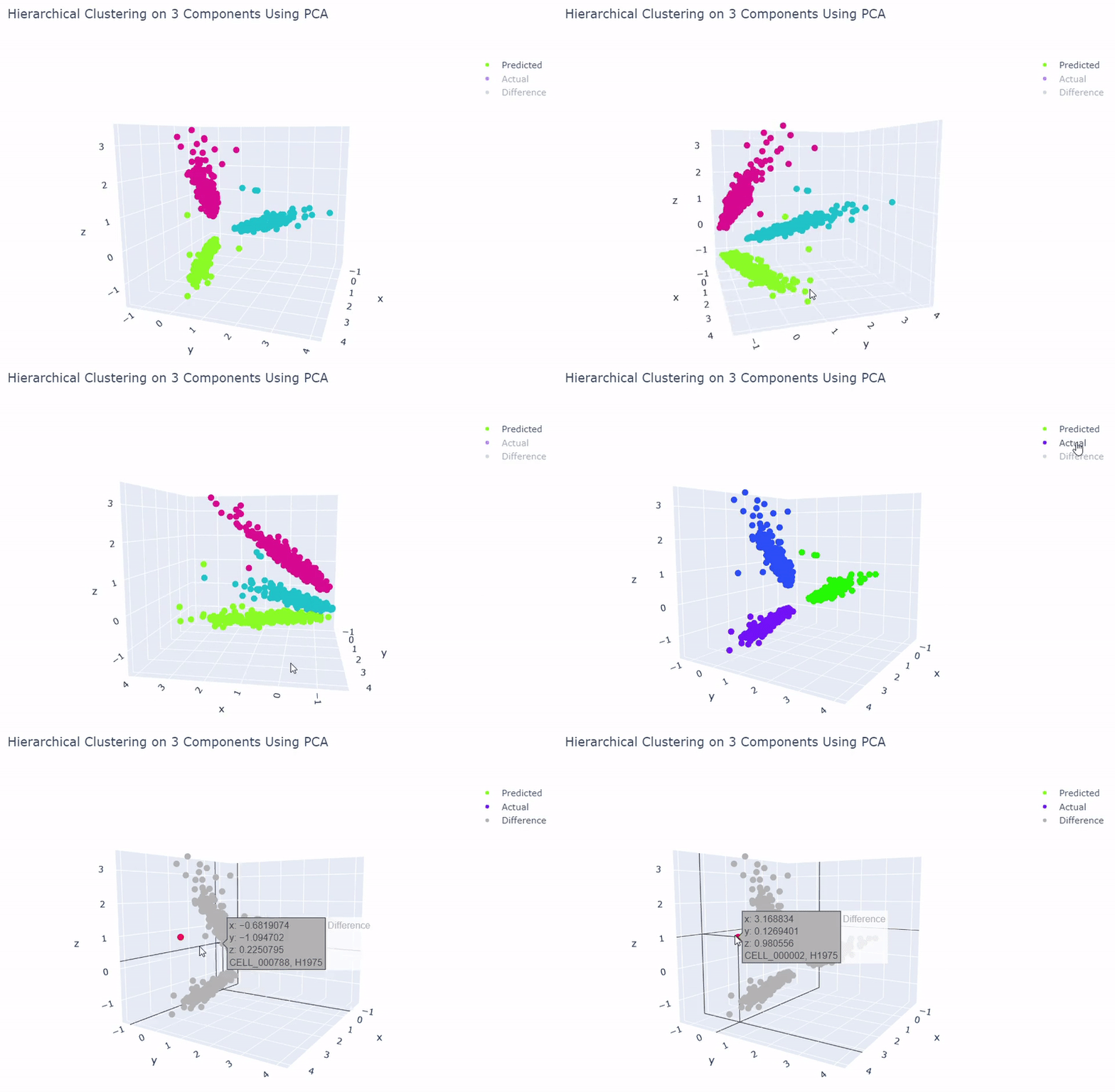
- Dataset originally named sc_10x by Tian et al.
- Contains human lung adenocarcinoma cancer cells with three cell lines
- Best accuracy was 99.9% in which 901 out of 902 cells were assigned to the correct cell line
- Use standardization and PCA or ICA with three components with agglomerative hierarchical clustering or BIRCH
Splat Simulated
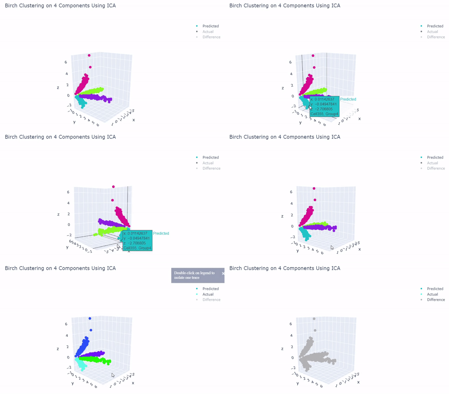
- Dataset of artificial data simulated with Splat during this project
- Gene expression imitates sc_10x
- Ground truth contains four target groups
- Was able to achieve 100% accuracy in which 2000 cells were correctly grouped
- Use standardization and PCA or ICA with four components along with agglomerative hierarchical clustering, BIRCH or mini batch k-means
Mouse Cortex
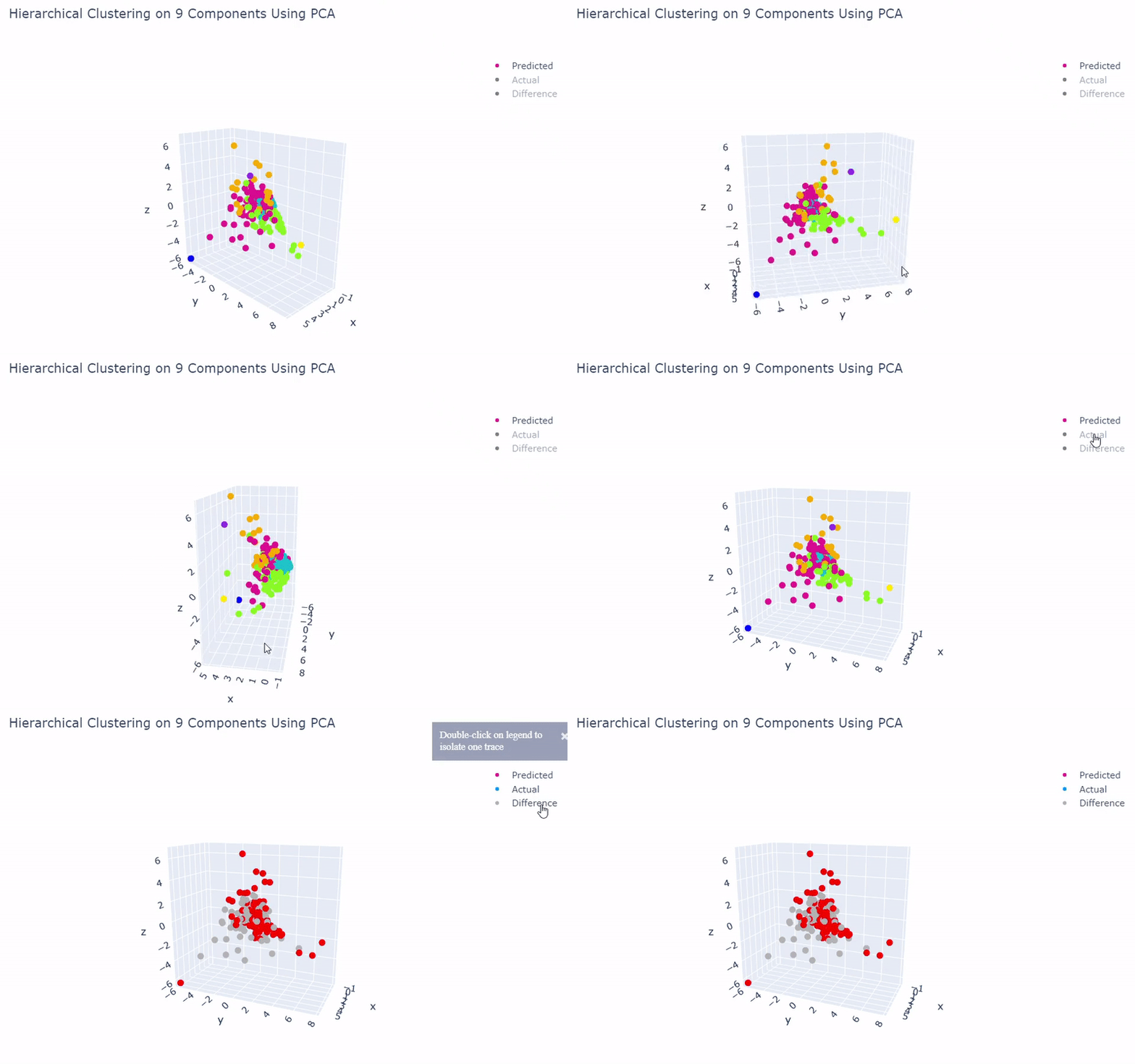
- Dataset originally named mouse cortex mRNA by Zeisel et al.
- Contains brain cells from mouse cortex and hippocampus with nine groups and 47 subgroups determined previously using BackSPIN biclustering
- Unfortunately I was only able to get 44% accuracy
- Standard clustering methods are not as reliable with this data as cells show an overlapping spectrum of gene expression
𝗧𝗼𝗽𝗼𝗹𝗼𝗴𝗶𝗰𝗮𝗹 𝗗𝗮𝘁𝗮 𝗔𝗻𝗮𝗹𝘆𝘀𝗶𝘀 𝘄𝗶𝘁𝗵 𝗞𝗲𝗽𝗹𝗲𝗿 𝗠𝗮𝗽𝗽𝗲𝗿
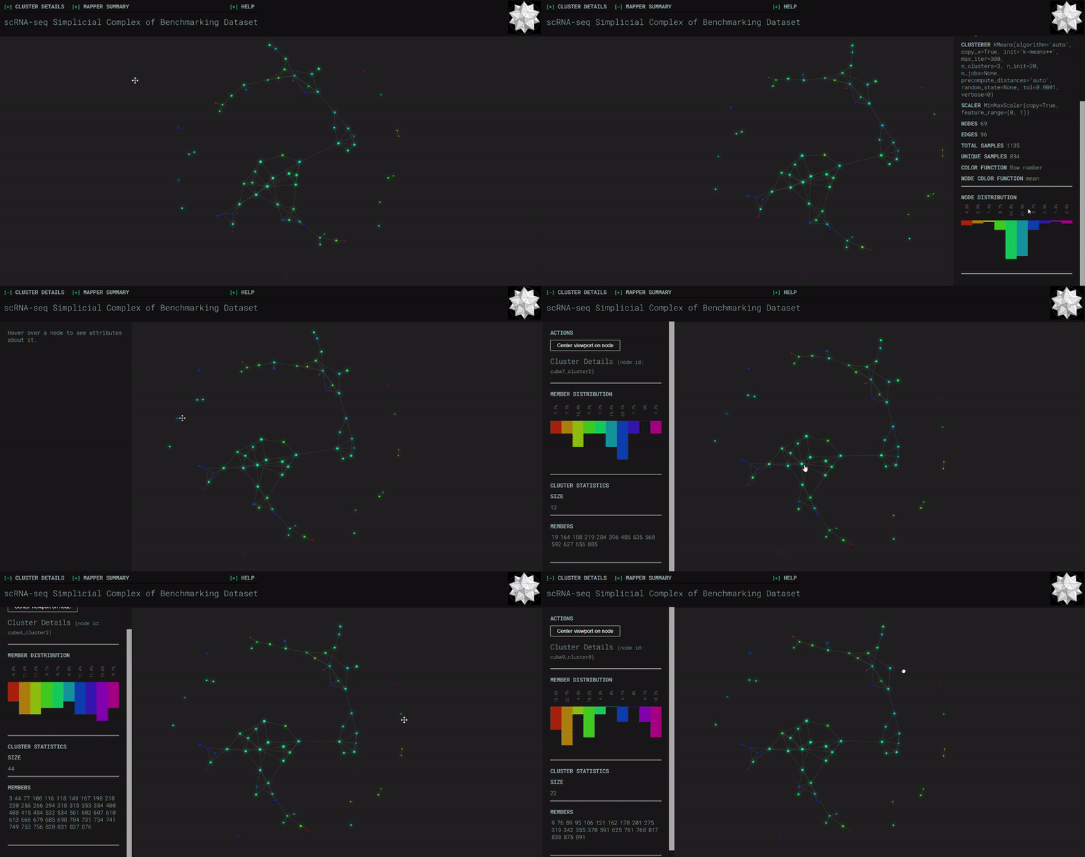
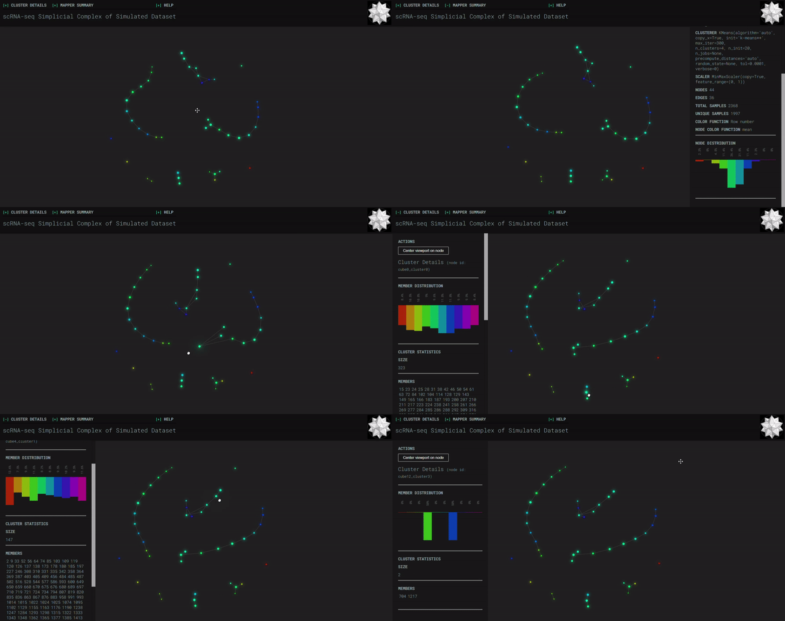
Simplicial complexes for each dataset were created with the same hyperparameters so that topological features can be compared.
Benchmark
Splat Simulated
Mouse Cortex

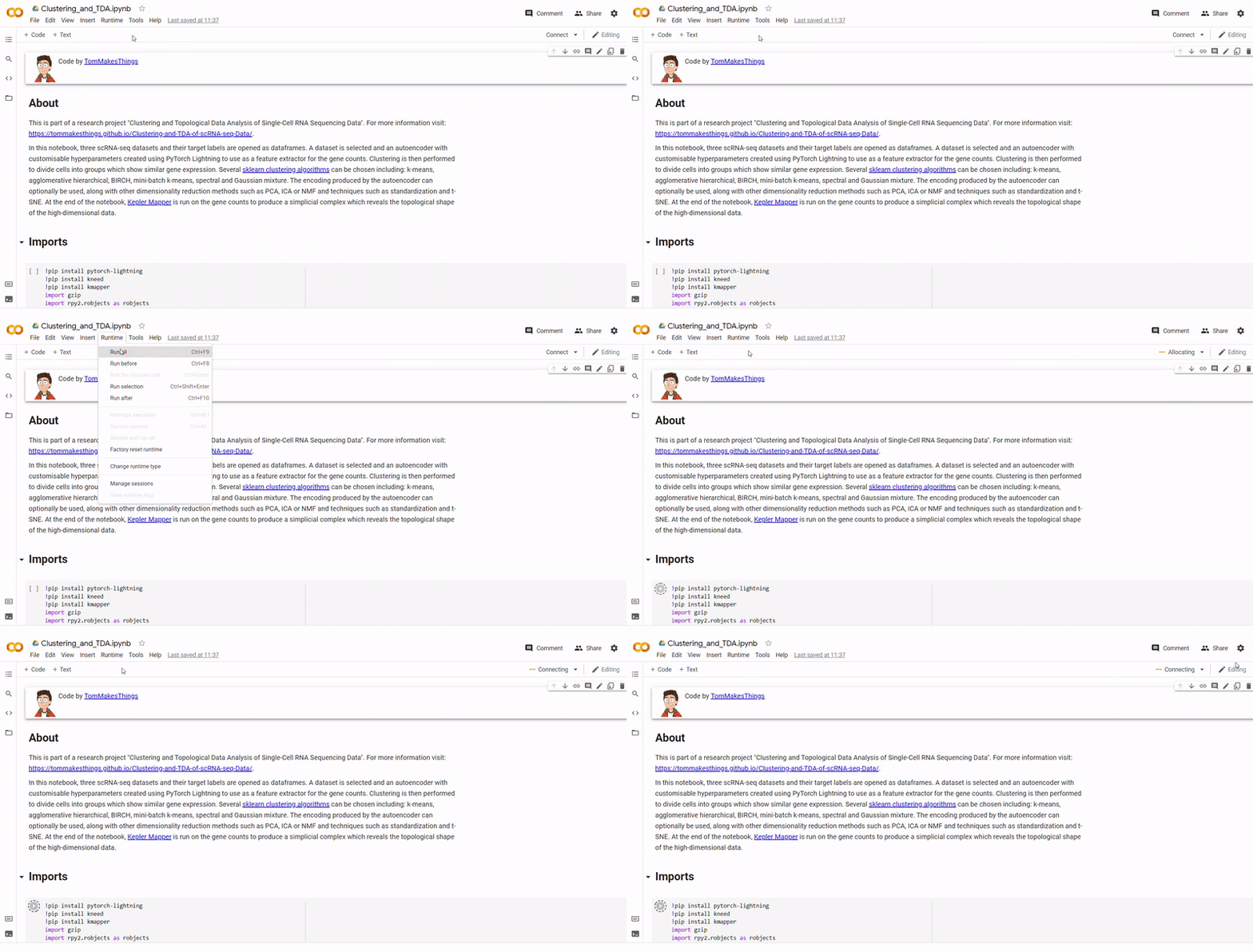
The code was written in Python and R across two Jupyter notebooks. For an explaination of each notebook, see the section below. These were developed in Google Colab which is a free Jupyter notebook environment that allows you to run code through a browser.
Click to Show Instructions
The repository consists of two branches: main and gh-pages. The contents of each branch is explained here.
Jupyter Notebooks
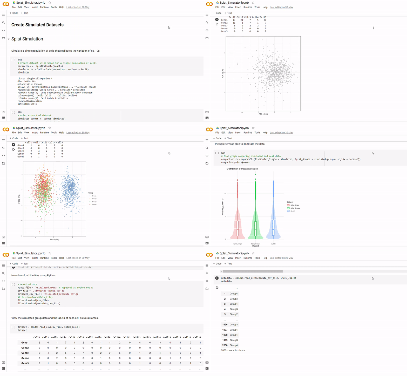
The purpose of notebook Splat_Simulator.ipynb is to produce new, artificial scRNA-seq data. For this project, it was used to create the simulated dataset, though can easily be altered to make new data for other purposes. To see a fully executed version of the code, click here.
- Gene counts and group labels are generated using the Splat simulator, which is part of the R package Splatter, and so the code contains a mix between Python and inline R.
- To mimick true biological gene expression, the benchmark dataset has been set to use as a seed, though this could be swapped out to imitate another dataset.
- After seeding the simulator, datapoints are generated with each belonging to one of four groups.
- The new data and labels are then saved as CSV files using Python. These can be downloaded and reopened to use in Clustering_and_TDA.ipynb.
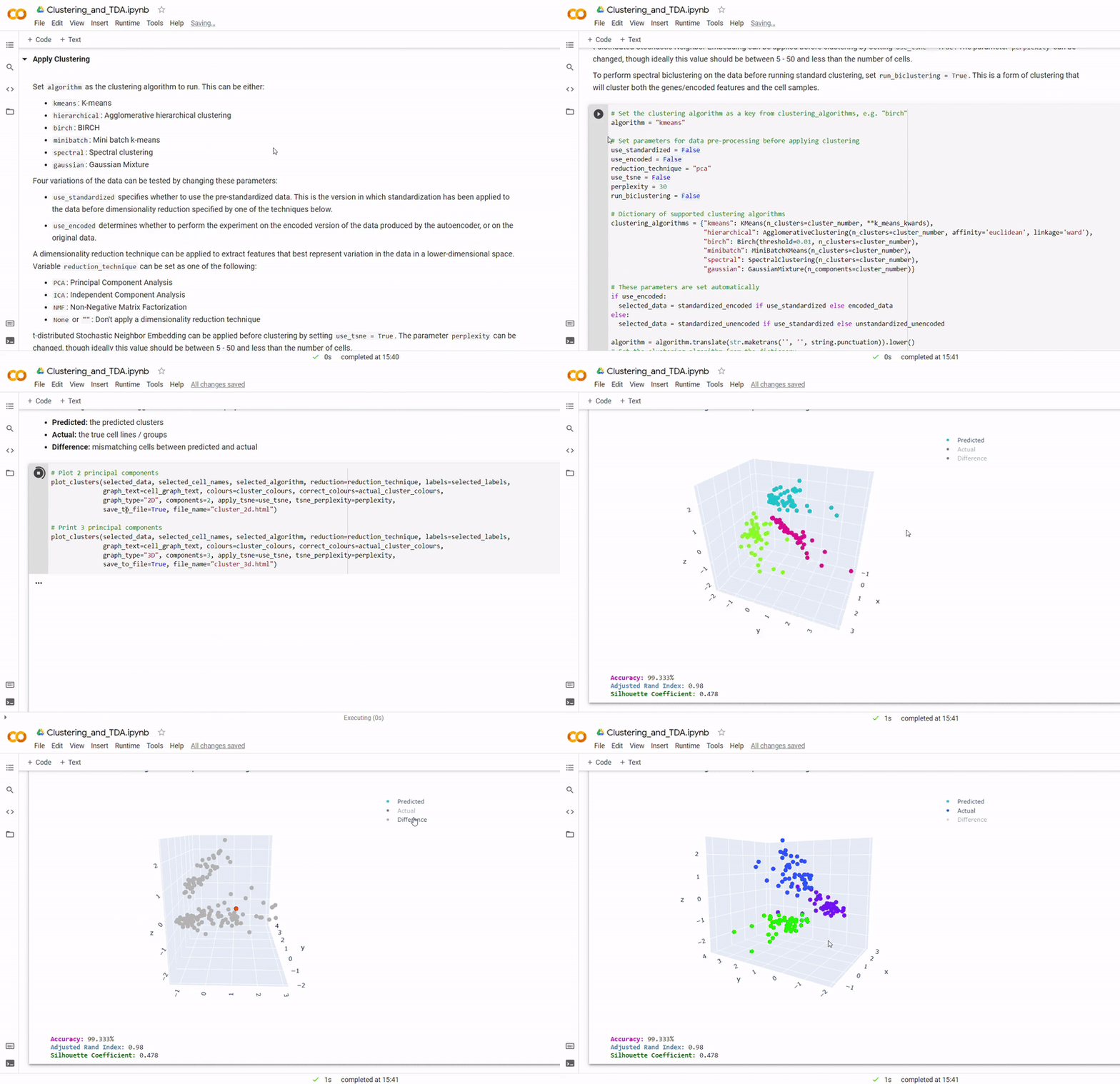
- First the datasets and their target labels are opened as dataframes. The given datasets are downloaded from URL so that the notebook can be run with no set up required, although the code has been designed so that it can also be run with your own dataset.
- Next, a dataset is selected and an autoencoder with customisable hyperparameters created using PyTorch Lightning to use as a feature extractor for the gene counts
- Then clustering is performed to divide cells into groups which show similar gene expression. Several clustering algorithms can be chosen including: k-means, agglomerative hierarchical, BIRCH, mini-batch k-means, spectral and Gaussian mixture. The encoding produced by the autoencoder can optionally be used, along with other dimensionality reduction methods such as PCA, ICA or NMF and techniques such as standardization and t-SNE.
- At the end of the notebook, Kepler Mapper is run on the gene counts to produce a simplicial complex to reveal the topological shape of the high-dimensional data.
In the notebook Clustering_and_TDA.ipynb, experimentation is performed on the three given datasets. To see a fully executed version of the code with interactive graphs, click here.
Data
This folder contains CSV, text and R object files containing the gene count data, labels and metadata for three scRNA-seq datasets. These are downloaded and opened automatically in notebook Clustering_and_TDA.ipynb.

To find out more about the datasets see the GitHub Pages site.
 These folders contain zip files that are opened automatically in notebook Clustering_and_TDA.ipynb. and do not need to be manually downloaded. These files allow the state of trained autoencoders to be reloaded for the three datasets to avoid training new models every time the notebook is run. Within each zip is a model checkpoint file containing the model weights, as well as text files listing the cells / samples selected for the testing, training and validation data to ensure training and testing data does not overlap when the notebook is run again.
Graphs
In this folder, interactive HTML graphs from experiments with clustering and topological data analysis are located.
- Target_Groups - graphs of expected cells lines / groups
- K-Means - experiments with k-means clustering
- Hierarchical_Clustering - experiments with agglomerative hierarchical clustering
- Alternative_Algorithms - experiments with other clustering algorithms
- Topological_Data_Analysis - simplicial complexes produced through Kepler Mapper
To view a particular graph, refer to the Graph Finder on the GitHub Pages site.
