Self-Driving Car Engineer Nanodegree Program
For this project we used a global kinematic model, which is a simplification of a dynamic model that ignores tire forces, gravity and mass.
The state model is represented by the vehicles position, orientation angle (in radians) and velocity.
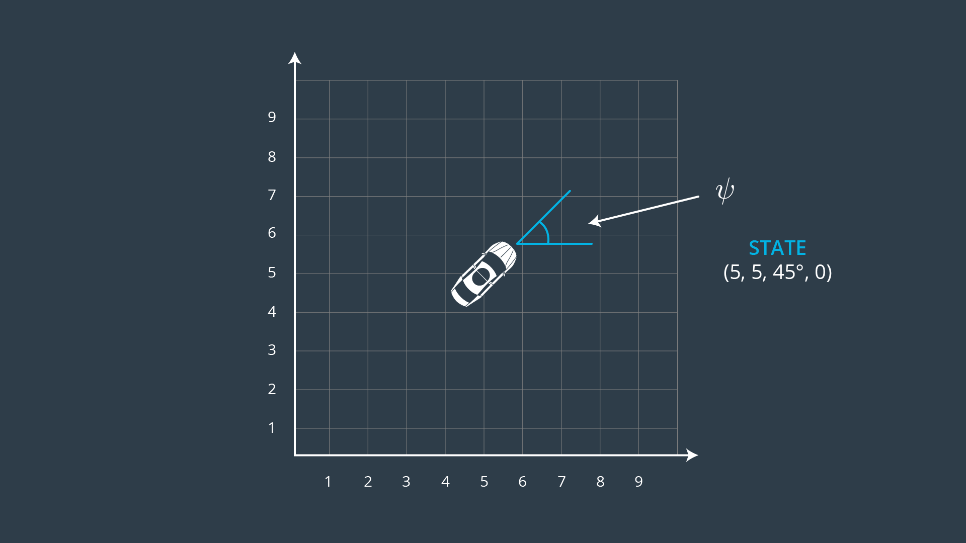
A cross track error (distance of vehicle from trajectory) and an orientation error (difference of vehicle orientation and trajectory orientation) were also included in the state model.
Two actuators were used, delta - to represent the steering angle (normalised to [-1,1]) and a - for acceleration corresponding to a throttle, with negative values for braking.
The simulator passes via a socket, ptsx & ptsy of six waypoints (5 in front, 1 near the vehicle), the vehicle x,y map position, orientation and speed (mph).
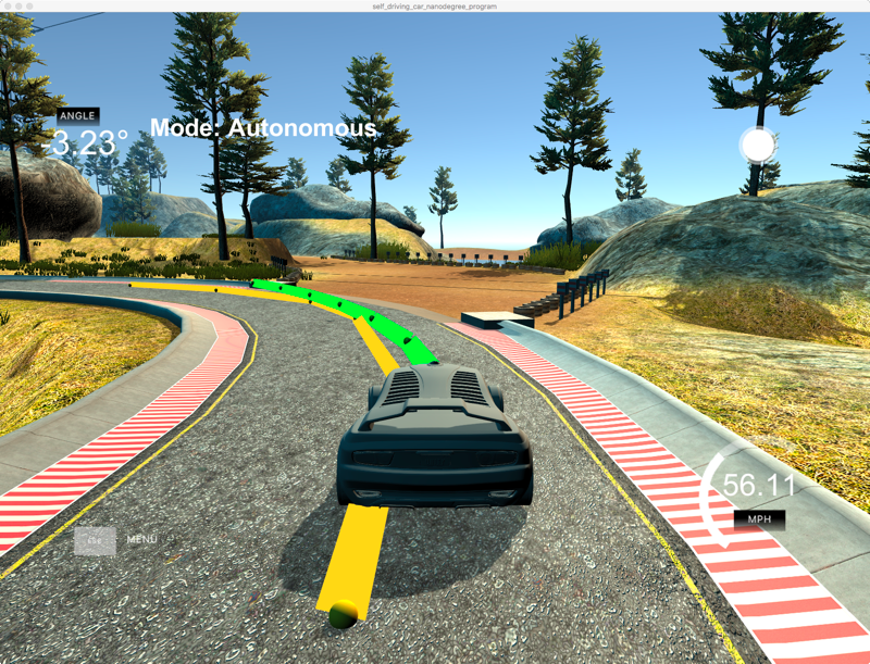
This data after being transformed into the vehicle map space, with new cross track error and orientation error calculated, is then passed into the MPC (Model Predictive Control) solve routine. It returns, the two new actuator values, with steering and acceleration (i.e. throttle) and the MPC predicted path (plotted in green in the simulator).
Constraint costs were applied to help the optimiser select an optimal update. Emphasis was placed on minimising orientation error and actuations, in particular steering (to keep the lines smooth).
   // Reference State Cost
    // TODO: Define the cost related the reference state and
    // any anything you think may be beneficial.
    // The part of the cost based on the reference state.
    for (int i = 0; i < N; i++) {
      fg[0] += CppAD::pow(vars[cte_start + i] - ref_cte, 2);
      fg[0] += 2 * CppAD::pow(vars[epsi_start + i] - ref_epsi, 2);
      fg[0] += CppAD::pow(vars[v_start + i] - ref_v, 2);
    }

    //
    // Setup Constraints
    //
    // NOTE: In this section you'll setup the model constraints.
    // Minimize the use of actuators.
    for (int i = 0; i < N - 1; i++) {
      fg[0] += CppAD::pow(vars[delta_start + i], 2);
      fg[0] += CppAD::pow(vars[a_start + i], 2);
    }

    // Minimize the value gap between sequential actuations.
    for (int i = 0; i < N - 2; i++) {
      fg[0] += 20000 * CppAD::pow(vars[delta_start + i + 1] - vars[delta_start + i], 2);
      fg[0] += 10 * CppAD::pow(vars[a_start + i + 1] - vars[a_start + i], 2);
    }
The MPC optimiser has two variables to represent the horizon into the future to predict actuator changes. They are determined by N (Number of timesteps) and dt (timestep duration) where T (time) = N * dt.
To help tune these settings, I copied the mpc_to_line project quiz, to a new project mpc_to_waypoint, and modified it to represent the initial state model to be used with the Udacity simulator. I was able to get good results looking out 3 seconds, with N = 15 and dt = 0.2. The following output are plots of 50 iterations from the initial vehicle state:
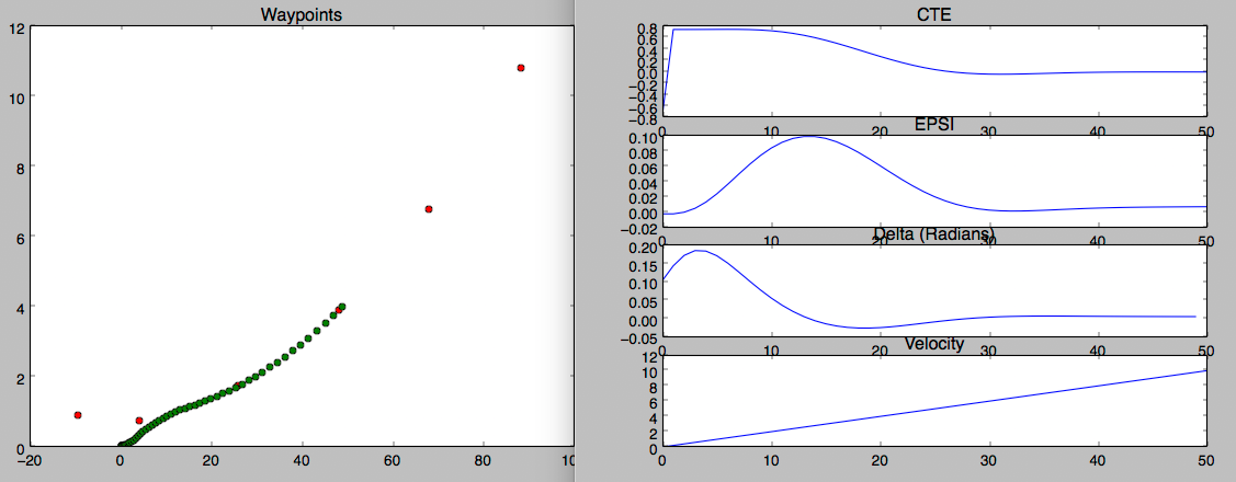
It seemed to be tracking quite nicely but speed was very slow.
However what I found, is that a horizon out 3 seconds in the simulator seemed to be too far. The faster the vehicle, the further forward the optimiser was looking. It shortly started to fail and the vehicle would end up in the lake or even worse airborne.
I tried reducing N and increasing dt. Eventually, via trial and error, I found good results where N was 8 to 10 and dt between ~0.08 to ~0.105. I eventually settled on calculating dt based on Time/N (with time set at ~.65 seconds and N on 8). If I saw the plotted MPC line coming close to the 2nd furthest plotted waypoint at higher speeds, it started to correspond, with the MPC optimiser failing.
The reference speed also played a part. To drive safely around the track, to ensure the project meets requirement, I kept it at 60 MPH.
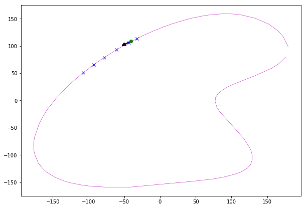
An example plot of the track with the first way points, vehicle position and orientation follows:
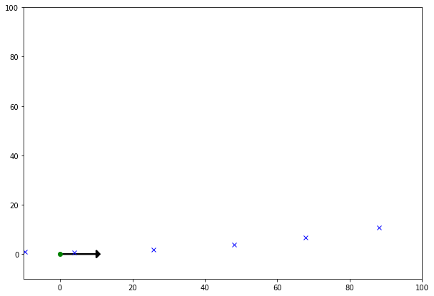
To make updating easier and to provide data to be able to draw, the waypoints and the predicted path from the MPC solver, coordinates were transformed into vehicle space. This meant also that the initial position of the vehicle state, for the solver was (0 + velocity in KPH * 100 ms of latency,0), which included a projection of distance travelled to cover latency, with a corresponding angle orientation of zero. These coordinates were used in the poly fit. It had an added benefit of simplifying, the derivative calculation required for the orientation error.
The following plot is the same waypoints transformed to the vehicle space map, with the arrow representing the orientation of the vehicle:
Before sending the result back to the simulator a 100ms latency delay was implemented.
this_thread::sleep_for(chrono::milliseconds(100));
This replicated the actuation delay that would be experienced in a real-world vehicle.
I experimented with trying to understand if the ratio of dt (time interval) to latency in seconds, being near 1 (i.e. the time interval was close to the latency value), had an impact on the ability of the MPC algorithm to handle latency. Anecdotal evidence supported that; but in reality ratio values of < 1 (for this project, I had (.65/8)/.100 = .0.8125) were the reality to ensure the optimiser was able to find a solution.
As described in the previous section, the vehicle position was projected forward, the distance it would travel, to cover 100ms of latency.
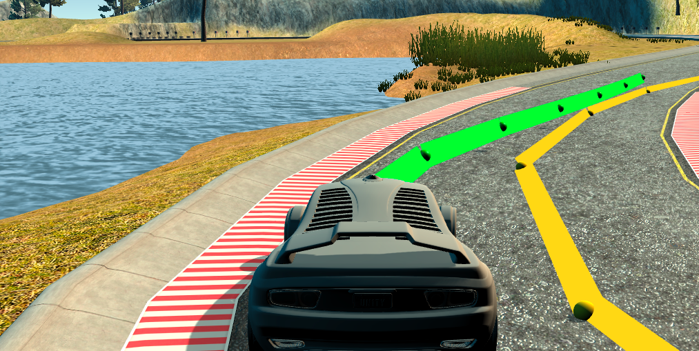
However before I implemented the forward projection for latency, you could see in places where the vehicle lagged a little in its turning. The MPC, however predicted the path correctly back onto the centre line of the track per following image:
After I implemented the latency projection calculation, the vehicle was able to stay closer to center, more readily per this image:
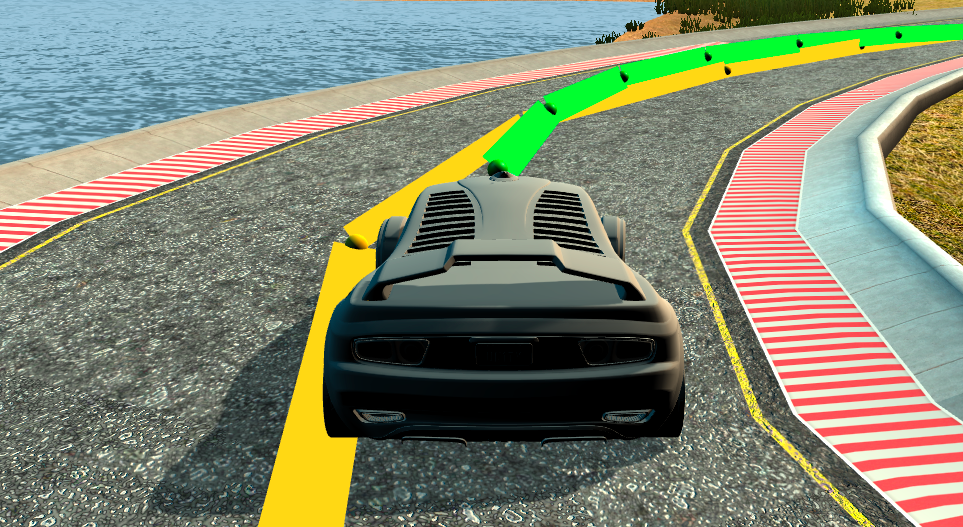
Over all the drive around this simulator track, was smoother and lacked steering wobbles, when compared to using a PID controller.
- cmake >= 3.5
- All OSes: click here for installation instructions
- make >= 4.1
- Linux: make is installed by default on most Linux distros
- Mac: install Xcode command line tools to get make
- Windows: Click here for installation instructions
- gcc/g++ >= 5.4
- Linux: gcc / g++ is installed by default on most Linux distros
- Mac: same deal as make - [install Xcode command line tools]((https://developer.apple.com/xcode/features/)
- Windows: recommend using MinGW
- uWebSockets == 0.14, but the master branch will probably work just fine
- Follow the instructions in the uWebSockets README to get setup for your platform. You can download the zip of the appropriate version from the releases page. Here's a link to the v0.14 zip.
- If you have MacOS and have Homebrew installed you can just run the ./install-mac.sh script to install this.
- Ipopt
- Mac:
brew install ipopt --with-openblas - Linux
- You will need a version of Ipopt 3.12.1 or higher. The version available through
apt-getis 3.11.x. If you can get that version to work great but if not there's a scriptinstall_ipopt.shthat will install Ipopt. You just need to download the source from the Ipopt releases page or the Github releases page. - Then call
install_ipopt.shwith the source directory as the first argument, ex:bash install_ipopt.sh Ipopt-3.12.1.
- You will need a version of Ipopt 3.12.1 or higher. The version available through
- Windows: TODO. If you can use the Linux subsystem and follow the Linux instructions.
- Mac:
- CppAD
- Mac:
brew install cppad - Linux
sudo apt-get install cppador equivalent. - Windows: TODO. If you can use the Linux subsystem and follow the Linux instructions.
- Mac:
- Eigen. This is already part of the repo so you shouldn't have to worry about it.
- Simulator. You can download these from the releases tab.
- Clone this repo.
- Make a build directory:
mkdir build && cd build - Compile:
cmake .. && make - Run it:
./mpc.
- It's recommended to test the MPC on basic examples to see if your implementation behaves as desired. One possible example is the vehicle starting offset of a straight line (reference). If the MPC implementation is correct, after some number of timesteps (not too many) it should find and track the reference line.
- The
lake_track_waypoints.csvfile has the waypoints of the lake track. You could use this to fit polynomials and points and see of how well your model tracks curve. NOTE: This file might be not completely in sync with the simulator so your solution should NOT depend on it. - For visualization this C++ matplotlib wrapper could be helpful.
We've purposefully kept editor configuration files out of this repo in order to keep it as simple and environment agnostic as possible. However, we recommend using the following settings:
- indent using spaces
- set tab width to 2 spaces (keeps the matrices in source code aligned)
Please (do your best to) stick to Google's C++ style guide.
Note: regardless of the changes you make, your project must be buildable using cmake and make!
More information is only accessible by people who are already enrolled in Term 2 of CarND. If you are enrolled, see the project page for instructions and the project rubric.
- You don't have to follow this directory structure, but if you do, your work will span all of the .cpp files here. Keep an eye out for TODOs.
Help your fellow students!
We decided to create Makefiles with cmake to keep this project as platform agnostic as possible. Similarly, we omitted IDE profiles in order to we ensure that students don't feel pressured to use one IDE or another.
However! I'd love to help people get up and running with their IDEs of choice. If you've created a profile for an IDE that you think other students would appreciate, we'd love to have you add the requisite profile files and instructions to ide_profiles/. For example if you wanted to add a VS Code profile, you'd add:
- /ide_profiles/vscode/.vscode
- /ide_profiles/vscode/README.md
The README should explain what the profile does, how to take advantage of it, and how to install it.
Frankly, I've never been involved in a project with multiple IDE profiles before. I believe the best way to handle this would be to keep them out of the repo root to avoid clutter. My expectation is that most profiles will include instructions to copy files to a new location to get picked up by the IDE, but that's just a guess.
One last note here: regardless of the IDE used, every submitted project must still be compilable with cmake and make./