DistMesh2D.jl

The package provides Julia implementation of DistMesh algorithm developed by Per-Olof Persson and Gilbert Strang allowing to generate meshes on 2D plane, using DelDir.jl which is a Julia wrapper for Delaunay triangulations and Voronoi/Dirichlet tessellations. Before using this package I highly recommend reading this document covering basic MATLAB's use-cases, because this packages tries to provide similar runtime interface to original one.

Installation

To use DistMesh2D.jl clone the repository and add it to the local package registry.

Usage

To generate a mesh, define a signed distance function, desired edge length function, bounding box, distance between points in initial distribution and run the meshing algorithm.

julia> fdistance(p) = sqrt(sum(p .^ 2)) - 1
fdistance (generic function with 1 method)

julia> fedgelength(p) = 1.0
fedgelength (generic function with 1 method)

julia> boundingbox = [-1.0 -1.0; 1.0 1.0]
2×2 Array{Float64,2}:
 -1.0  -1.0
  1.0   1.0

julia> initdistance = 0.2
0.2

julia> x, y = distmesh2d(fdistance, fedgelength, boundingbox, initdistance)
([-0.8408297336717067, -0.6993829085766673, NaN, -0.5315455685570857, -0.6993829085766673, NaN, -0.5822722080639808, -0.6993829085766673, NaN, -0.5822722080639808  …  NaN, -0.60618605865758, -0.36756281453508466, NaN, -0.60618605865758, -0.7846917737263828, NaN, -0.60618605865758, -0.5633752938295506, NaN], [-0.5412996931425073, -0.7147471921795109, NaN, -0.8470296986801119, -0.7147471921795109, NaN, -0.5521369576265936, -0.7147471921795109, NaN, -0.5521369576265936  …  NaN, 0.795322867083831, 0.92999869760509, NaN, 0.795322867083831, 0.6198861346071187, NaN, 0.795322867083831, 0.5800262182849156, NaN])

The output of a given function are points that are ready to be plotted with one of the available plotting libraries.

julia> using Gadfly

julia> Gadfly.plot(x = x, y = y, Geom.path, Coord.cartesian(fixed = true))

The output mesh

Generating more complex meshes

Library provides simple generic signed distance functions to define popular shapes like dcircle and drectangle.

function drectangle(
    p,
    x1::T,
    x2::T,
    y1::T,
    y2::T,
)::T where {T<:Float64}
    return -min(min(min(-y1 + p[2], y2 - p[2], -x1 + p[1], x2 - p[1])))
end

function dcircle(
    p,
    xc::T,
    yc::T,
    r::T
)::T where {T<:Float64}
    return sqrt((p[1] - xc) .^ 2 + (p[2] - yc) .^ 2) - r
end

Library provides simple operations on shapes like union, difference and intersections with via functions like dunion ddiff and dintersect. In each definition p is considered point. Other parameters are proper signed distance functions.

function dunion(
    p,
    dfs::Function...,
)::Float64
    return min([fun(p) for fun in dfs]...)
end

function ddiff(
    p,
    d1::Function,
    dfs::Function...
)::Float64
    return max(d1(p), [-fun(p) for fun in dfs]...)
end

function dintersect(
        p,
        dfs::Function...
)::Float64
    return max([fun(p) for fun in dfs]...)
end

Other useful functions are huniform which provides uniform height distribution for point p and protate which rotates given point by passed value.

function huniform(p)::Float64
    return ones(size(p, 1), 1)[1]
end

function protate(p,phi)
    return p*[cos(phi) -sin(phi); sin(phi) cos(phi)]
end

Non-uniform height function

Meshes with non uniform height functions also can be easily plotted. First we define signed distance functions which in this example is a rectangle with circle hole inside.

julia> outrect(p) = drectangle(p, -100.0, 100.0, -100.0, 100.0)
outrect (generic function with 1 method)

julia> incircle(p) = dcircle(p, 0.0, 0.0, 40.0)
incircle (generic function with 1 method)

julia> fd(p) = ddiff(p, outrect, incircle)
fd (generic function with 1 method)

Then we define height functions which is not going to return the same value for every input parameters, but will give finer resolution closer to the circle.

julia> fh(p) = min(4 * sqrt(sum(p.^2)) - 100)
fh (generic function with 1 method)

Next we define a bounding box bbox that can fit our rectangle and a value representing distance between points in initial distribution.

julia> bbox = [-100.0 -100.0; 100.0 100.0]
2×2 Array{Float64,2}:
 -100.0  -100.0
  100.0   100.0

julia> h0 = 10.0
10.0

To let the rectangle withstand the triangulation we need to defined its corner points as fixed.

julia> pfix = [-100.0 -100.0; -100.0 100.0; 100.0 -100.0; 100.0 100.0]
4×2 Array{Float64,2}:
 -100.0  -100.0
 -100.0   100.0
  100.0  -100.0
  100.0   100.0

Finally we define the dptol parameter which represents the limit value. Algorithms will loop as long as all movements, relative to bar lengths in given iteration are not below it.

julia> dptol = 0.003
0.003

julia> x, y = distmesh2d(fd, fh, bbox, h0, pfix=pfix, dptol=dptol)
([-100.0, -76.71718215838415, NaN, -62.29844095886764, -76.71718215838415, NaN, -100.0, -76.71718215838415, NaN, -100.0  …  NaN, 100.0, 100.0, NaN, 100.0, 78.01048490854643, NaN, 100.0, 80.72224653575613, NaN], [-80.56252474196684, -77.31440723125387, NaN, -62.263859671319544, -77.31440723125387, NaN, -65.15571042094268, -77.31440723125387, NaN, -65.15571042094268  …  NaN, 79.78462487451092, 63.972558404391755, NaN, 79.78462487451092, 76.7946778947107, NaN, 79.78462487451092, 100.0, NaN])

julia> Gadfly.plot(x = x, y = y, Geom.path, Coord.cartesian(fixed = true))

The output mesh

Composing shapes

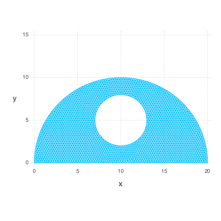
Let's say we want to mesh a simplified version of R2D2 head. By "simplified" I mean a semicircle with a hole in the center. We are going to work on bbox = [0.0 0.0; 20.0 10.0] and h0 = 0.25. First we define the hole as a small circle.

julia> sc(p) = dcircle(p, 10.0, 5.0, 3.0)
sc (generic function with 1 method)

Then we define a bigger circle.

julia> bc(p) = dcircle(p, 10.0, 0.0, 10.0)
bc (generic function with 1 method)

Next we want the smaller circle to stay empty during triangulation so we calculate the difference between functions.

julia> fds(p) = ddiff(p, bc, sc)
fds (generic function with 1 method)

Finally we define a rectangle and calculate its intersection with the area represented by the fds function.

julia> dr(p) = drectangle(p, 0.0, 20.0, 0.0, 10.0)
dr (generic function with 1 method)

julia> fd(p) = dintersect(p, dr, fds)
fd (generic function with 1 method)

We also need two fixed points.

julia> pfix = [0.0 0.0; 20.0 0.0]
2×2 Array{Float64,2}:
  0.0  0.0
 20.0  0.0

Finally we mesh our distance, passing additional logmi parameter with value equal to true. This parameter slows down the algorithm, but turns on logging of the minimal move index value that occured in all triangulations so far. Monitoring minimal move index is helpful to determine whether the algorithm is going forward and closer to dptol which by default is equal to 0.001.

julia> x, y = distmesh2d(fd, huniform, bbox, h0, pfix=pfix, logmi=true)
[ Info: Minimal move index is 1.7848378957838162
[ Info: Minimal move index is 0.6341210762677251
[ Info: Minimal move index is 0.3189998493116862
.
.
.
.
[ Info: Minimal move index is 0.0010124268021825809
[ Info: Minimal move index is 0.0010102509818988507
[ Info: Minimal move index is 0.0010080823842259872
[ Info: Minimal move index is 0.0010059209713983509
[ Info: Minimal move index is 0.0010037667055315528
[ Info: Minimal move index is 0.0010016195522329304
([0.39168705623677563, 0.24949716765305802, NaN, 1.4066677906807563, 1.1484883086226838, NaN, 2.089037409389501, 1.9403068274377, NaN, 1.6763442046107901  …  NaN, 5.225956577772305, 5.45051039916194, NaN, 5.225956577772305, 4.9344362730766385, NaN, 5.225956577772305, 5.523495989156209, NaN], [2.063690666551136, 2.2198411283347967, NaN, 1.619386786583647, 1.6285058990860535, NaN, 0.0, 0.23721296745446183, NaN, 0.23008747967549248  …  NaN, 8.786837276630676, 8.730320688506946, NaN, 8.786837276630676, 8.622068433075366, NaN, 8.786837276630676, 8.942086553129595, NaN])

The output mesh

Error handling

Considering the fact that this package relies on DelDir.jl to triangulate points, some errors occurring in triangulation process can be hard to solve, because they can occur in original triangulation package itself. Those errors are caught, wrapped and exposed to the user with information about iteration, triangulated dataset and inner error itself. Supposing we changed bbox and h0 from previous example to:

julia> bbox = [0.0 0.0; 10.0 10.0]
2×2 Array{Float64,2}:
  0.0   0.0
 10.0  10.0

julia> h0 = 2.5
2.5

Which means that the current area defined by bbox is too small to triangulate points. We are going to face the following error.

julia> x, y = distmesh2d(fd, huniform, bbox, h0, pfix=pfix)
ERROR: Triangulation failed with given data: 
 Points = [0.125 0.21650635094610965; 0.375 0.21650635094610965; 0.25 0.4330127018922193; 0.375 0.649519052838329; 0.625 0.21650635094610965; 0.5 0.4330127018922193; 0.625 0.649519052838329; 0.875 0.21650635094610965; 0.75 0.8660254037844386; 1.125 0.21650635094610965; 1.0 0.8660254037844386] 
 Iteration = 0 
 Inner error = DomainError([0.0, 1.0, 0.0, 1.0], "Boundary window is too small")
Stacktrace:
 [1] distmesh2d(::typeof(fd), ::typeof(huniform), ::Array{Float64,2}, ::Float64; pfix::Array{Float64,2}, dptol::Float64, ttol::Float64, geps::Float64, Fscale::Float64, deltat::Float64, deps::Float64, logmi::Bool) at /Users/jstarczewski/GitProjects/DistMesh2D.jl/src/distmesh.jl:33
 [2] top-level scope at none:1
julia> 

Note that when filling an issue it is highly recommended to check whether the error comes from meshing algorithm or directly from triangulation.