EVA

EVA S8 notes:

Building the architecture of Resnet - 18

1. A basic resnet architectue is built using the concepts of Resnet 18 as available in the documentation. The same is shown below.
   
2. This architecture of resnet has been modified by passing it through a custsom built class to break down the network to extract the convolution at the level of 8x8 channel output, which is at the 3th block. This is preferred so that the heat map superimposition may be significantly big enough to understand the learning of the model.
   
   
3. A backward hook is incorporated at the fourth block layer. The rest of the network is the same. Max pooling layer has been applied before the classification layer to accomodate for the dimensions of the image.
   
   
4. The following are the modifications of the network.
   

• Layer normalization at every layer of the architecture
  
  
• Incoproration of Reduce Learning rate on Plateau which is implemented at the end of every epoch.
  -
  
• Incorporation of augmemntation techinques such as rotate(+/-5), Cutout (16x16), and random crop of the images.
  
  

5. Training is done for 40 epochs.
   
   

6. The training and validation losses/accuracy for 40 epochs is as shown below
   
   

7. The misclasified images are plotted using a custom class built and the heat map of the grad cam is plotted againt the images. The heat map shows which part of the image the model has identified to miclassify the image. Since the images are of low definition the clarity of the grad cam may not be well established and explained. However the same may be utilized to classify higher quality images.
   

8. The amount of gradient in the heat cam to be applied or super imposed on the original image may be varied by using a hyperpara

9. Some concepts to understand here are as follows:-

Momentum:

Momentum is a concept in analog physics. Generally speaking, the momentum of an object refers to the tendency of the object to keep moving in the direction of its motion, which is the product of the mass and speed of the object.

Here’s a popular story about momentum: gradient descent is a man walking down a hill. He follows the steepest path downwards; his progress is slow, but steady. Momentum is a heavy ball rolling down the same hill. The added inertia acts both as a smoother and an accelerator, dampening oscillations and causing us to barrel through narrow valleys, small humps and local minima.

This standard story isn’t wrong, but it fails to explain many important behaviors of momentum. In fact, momentum can be understood far more precisely if we study it on the right model. [distill]

One nice model is the convex quadratic. This model is rich enough to reproduce momentum’s local dynamics in real problems, and yet simple enough to be understood in closed form. This balance gives us powerful traction for understanding this algorithm.

We begin with gradient descent. The algorithm has many virtues, but speed is not one of them. It is simple — when optimizing a smooth function f, we make a small step in the gradient w (k+1) = w( k) − α * ∇ f (w (k) )

For a step-size small enough, gradient descent makes a monotonic improvement at every iteration. It always converges, albeit to a local minimum. And under a few weak curvature conditions it can even get there at an exponential rate.

But the exponential decrease, though appealing in theory, can often be infuriatingly small. Things often begin quite well — with an impressive, almost immediate decrease in the loss. But as the iterations progress, things start to slow down. You start to get a nagging feeling you’re not making as much progress as you should be (so true 😑). What has gone wrong?

The problem could be the optimizer’s old nemesis, pathological curvature. Pathological curvature is, simply put, regions of f which aren’t scaled properly. The landscapes are often described as valleys, trenches, canals and ravines. The iterates either jump between valleys, or approach the optimum in small, timid steps. Progress along certain directions grind to a halt. In these unfortunate regions, gradient descent fumbles.

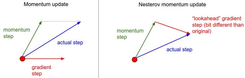
Momentum proposes the following tweak to gradient descent. We give gradient descent a short-term memory:

​ z (k+1) = β * z(k) + ∇ f (w(k))

​ w (k+1) = w( k) − α * z(k+1)

The change is innocent, and costs almost nothing. When β=0, we recover gradient descent. But forβ*=0.99 this appears to be the boost we need. Our iterations regain that speed and boldness it lost, speeding to the optimum with a renewed energy.

Optimizers call this minor miracle “acceleration”.

Simple Moving Average:

For a simple moving average, the formula is the sum of the data points over a given period divided by the number of periods.

MA=(P1+ P2 +P3 + P4 + P5)/5 --> An example of simple moving average for 5 points. When next point comes in, simply move the window (still taking in 5 point) so that (P2 + P3 + P4 + P5 + P6)/5 becomes new value for moving average.

Using moving averages is an effective method for eliminating strong fluctuations. The key limitation is that data points from older data are not weighted any differently than new data points. This is where weighted moving averages come into play.

Weighted Moving Average:

This approach assign a heavier weighting to more current data points since they are more relevant than data points in the distant past. The sum of the weighting should add up to 1 (or 100 percent). In the case of the simple moving average, the weightings are equally distributed.

Example:

WMA = (Price1×n + Price2×(n−1) + ⋯ Price n) / (n/2×(n+1))

where: n=Time period

Exponentially Weighted Moving Average:

Exponentially weighed averages deal with sequences of numbers.

That sequence V is the one plotted yellow above.

We’re approximately averaging over last 1 / (1- beta) points of sequence.

As you can see, with smaller numbers of beta, the new sequence turns out to be fluctuating a lot, because we’re averaging over smaller number of examples and therefore are ‘closer’ to the noisy data. With bigger values of beta, like beta=0.98, we get much smother curve, but it’s a little bit shifted to the right, because we average over larger number of example(around 50 for beta=0.98). Beta = 0.9 provides a good balance between these two extremes.

SGD with Momentum:

Where L — is loss function, triangular thing — gradient w.r.t weight and alpha — learning rate

Nesterov accelerated gradient:

Why momentum really works:

One major reason is: when we perform SGD, (mini-batch in reality as we choose batch size to speed up process instead of one image at a time), we are not computing the exact derivative of our actual loss function as we are estimating it on a small batch at a time and not the entire dataset. Thus the derivatives are kind of noisy to say which makes it difficult for network to learn.

Adding exponential weighted average kind of smoothes out the average and thus helps to provide better estimate as it includes average over previous calculated average.

The other reason lies in ravines. Ravine is an area, where the surface curves much more steeply in one dimension than in another. Ravines are common near local minimas in deep learning and SGD has troubles navigating them. SGD will tend to oscillate across the narrow ravine since the negative gradient will point down one of the steep sides rather than along the ravine towards the optimum. Momentum helps accelerate gradients in the right direction. below image 1 vs image 2(with momentum)

---