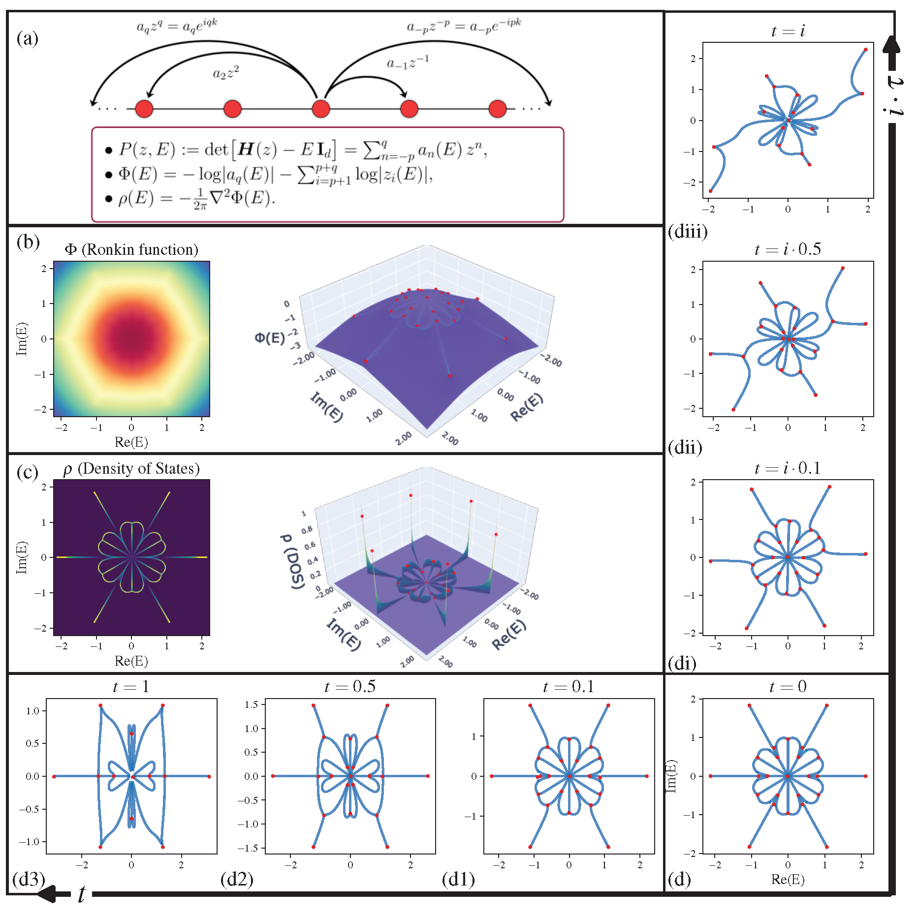
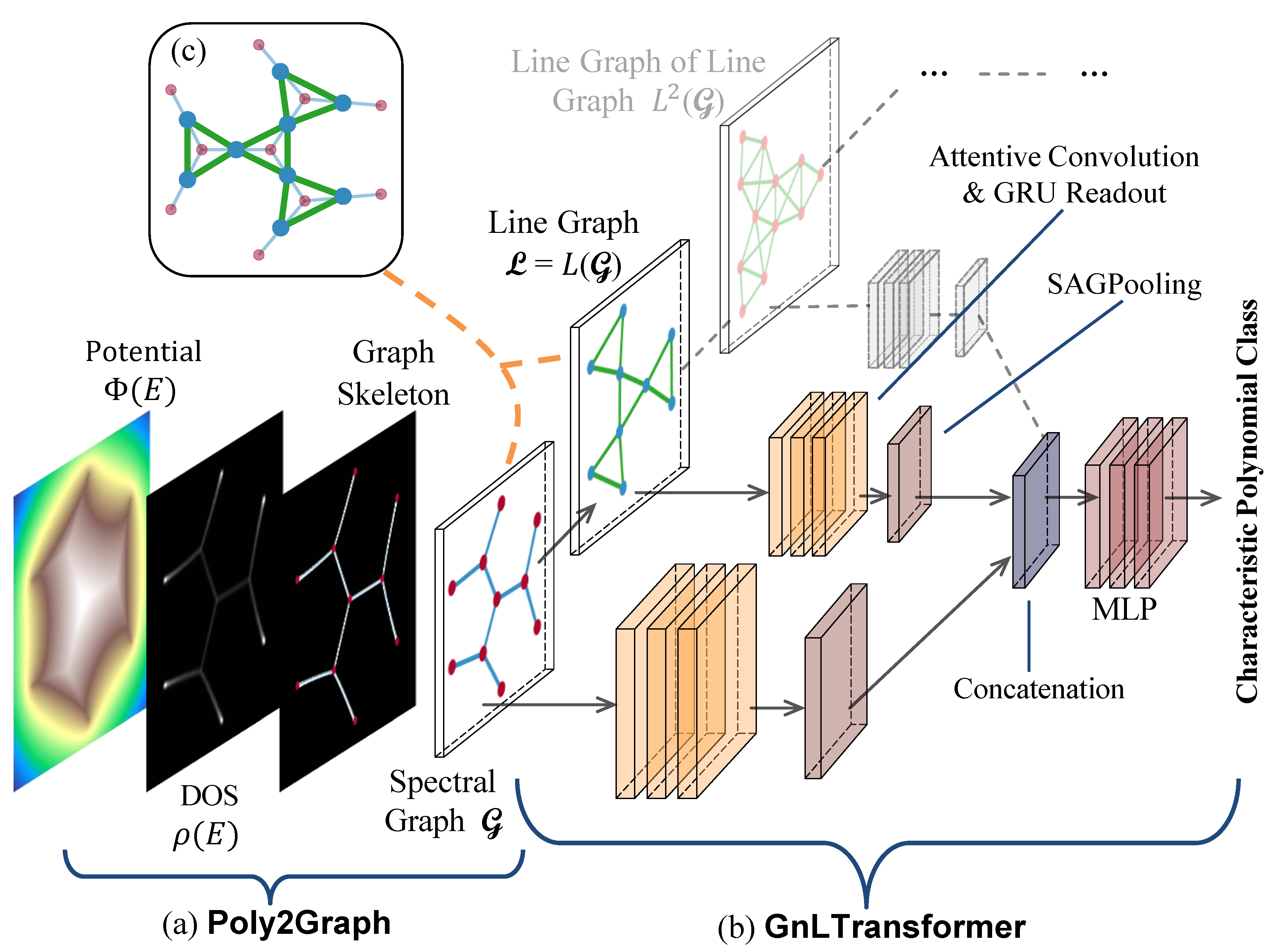
Poly2Graph & GnLTransformer

Poly2Graph is a Python package for automatic non-Hermitian spectral graph construction. It takes in the characteristic polynomial and returns the spectral graph.

Topological physics is one of the most dynamic and rapidly advancing fields in modern physics. Conventionally, topological classification focuses on eigenstate windings, a concept central to Hermitian topological lattices (e.g., topological insulators). Beyond such notion of topology, we unravel a distinct and diverse graph topology emerging in non-Hermitian systems' energy spectra, featuring a kaleidoscope of exotic shapes like stars, kites, insects, and braids. The spectral graph solely depends on the algebraic form of characteristic polynomial.

GnLTransformer is an explainable graph neural network that integrates multi-head attention mechanism and leverages line graphs as dual channels to explicitly capture higher-order relationships beyond node-node interactions.

Features

• Poly2Graph

  1. Fast construction of spectral graph from characteristic polynomial
  2. Support for one-band and multi-band systems
  3. Adaptive resolution for spectral potential calculation (one-band only)
  4. Automatic Spectral Boundary Determination (one-band only)
  5. Convert skeletonized image to its graph representation
  6. Dataset generation (one-band only)
  7. Visualization of spectral potential, density of states, and spectral graph

• GnLTransformer

  1. Line graph as dual channels. Extensible to capture any higher-order relationships.
  2. Explainability: Multi-head attention
  3. Visualization of node & edge attention weights and embedding similarity matrices

Installation

First make sure you have installed tensorflow pytorch, and torch_geometric according to your machine specifics. This module is tested on Python 3.9~3.12, tensorflow >=2.10, torch >=2.4 + cu121, and torch_geometric >=2.6.

tensorflow (CPU version is enough) is required for the optimization of poly2graph. GnLTransformer is written in pytorch and torch_geometric.

You can install the package via pip:

$ pip install poly2graph

or clone the repository and install it manually:

$ git clone https://github.com/sarinstein-yan/poly2graph.git
$ cd poly2graph
$ pip install -e . # or turn off the editable mode running `pip install .`

Check the installation:

import poly2graph as p2g
print(p2g.__version__)

Usage

See the Poly2Graph Tutorial JupyterNotebook.

Here we only list the core few functionalities.

One-band Spectral Graph

Take a one-band characteristic polynomial as an example:

$$P(E,z) = -z^{-2} - E - z + z^4$$

its coefficient list is c = [0, 0, -1, 0, 0, -1, 0, 0, 1]. poly2graph only takes in symmetric coefficient list where the middle element is the constant term (i.e. the coefficient of $z^0$). This is how poly2graph identifies the degree range. Note that the $-E$ term appearing as an addition to the constant term is the same for all one-band systems; thus there's no need to specify it. poly2graph automatically takes care.

### coefficient list (symmetrically formatted)
c = np.array([0, 0, -1, 0, 0, -1, 0, 0, 1])

Call spectral_graph with the coefficient list c and the energy range E_max, it will return the spectral graph as a networkx multigraph object.

The complex energy domain should be square grid that contains the spectral graph. The parameter E_max could be a list of 4 real numbers that specifies

[Re(E)_min, Re(E)_max, Im(E)_min, Im(E)_max]

or a single real number which will be interpreted as

E_max = Re(E)_max = Re(E)_min = Im(E)_max = Im(E)_min

Tip

The recommended way is to call auto_Emaxes to automatically determine the energy range (but so far it only supports one-band polynomial). Pass c as a numpy.array; otherwise, numba will raise an error.

### automatic boundaries of the energy grid
# `c` should be numpy array if `auto_Emaxes` is called
# otherwise numba will raise an error
E_maxes = p2g.auto_Emaxes(c)
print('Re(E) (min):', E_maxes[0], '  Re(E) (max):', E_maxes[1])
print('Im(E) (min):', E_maxes[2], '  Im(E) (max):', E_maxes[3])

### spectral graph
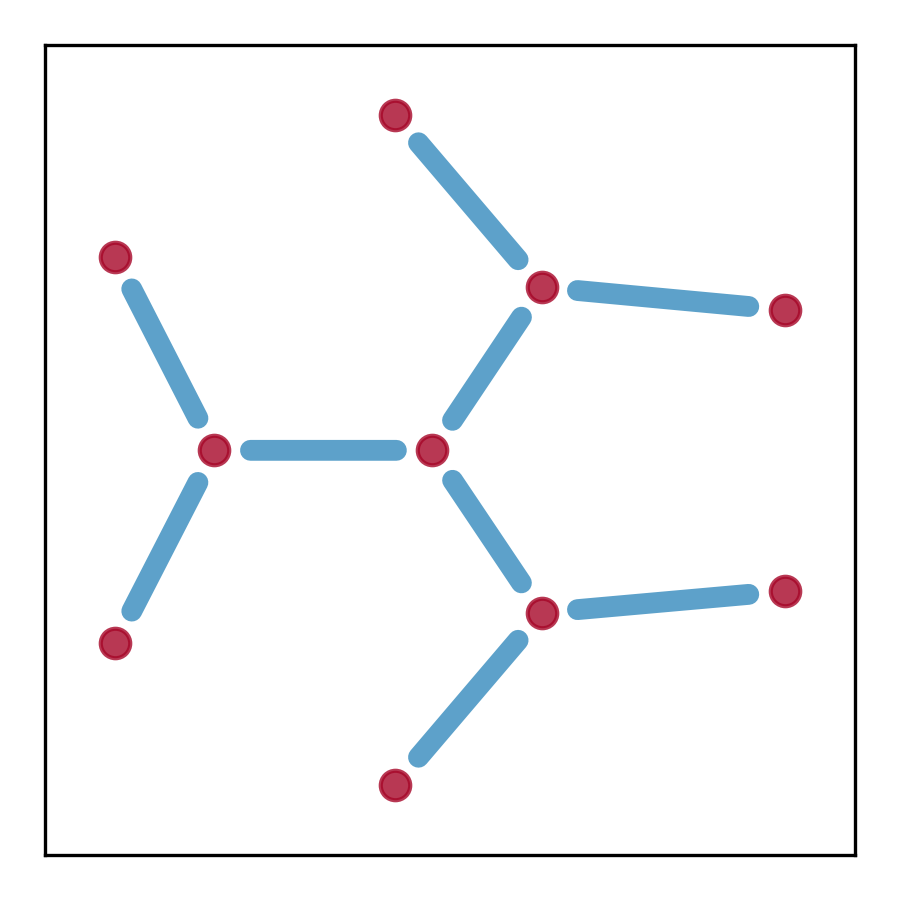
sg = p2g.spectral_graph(c, E_max=E_maxes)
print('\nObject type:', type(sg))

### plot spectral graph
fig, ax = plt.subplots(figsize=(3, 3))
pos_dict = {i[0]: (i[1][1], i[1][0]) for i in sg.nodes(data='o')}
nx.draw_networkx(sg, pos=pos_dict, ax=ax,
                 node_size=50, node_color='#A60628', with_labels=False, 
                 width=5, edge_color='#348ABD')
plt.show()

Re(E) (min): -2.4020020322545883   Re(E) (max): 2.5671486238803536
Im(E) (min): -2.4845753280674696   Im(E) (max): 2.4845753280674723

Object type: <class 'networkx.classes.multigraph.MultiGraph'>

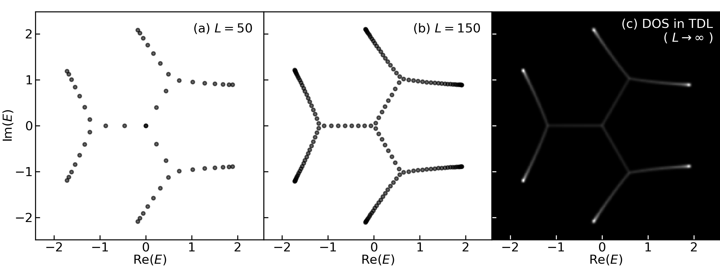
Let us diagonalize a real-space Hamiltonian to verify the spectral graph overlaps with the energy spectrum in thermodynamic limit ($L\to\infty$), and visualize the density of states (DOS) in TDL (see the companion paper for details).

The DOS, $\rho(E)$, is proportional to the lapaclacian of the spectral potential, $\Phi(E)$:

$$\rho(E) = -\frac{1}{2\pi} \Delta \Phi(E)$$

$\Delta = \partial_{\text{Re} E}^2 + \partial_{\text{Im} E}^2$ is the Laplacian operator on the complex energy plane. Laplacian operator extracts curvature; thus, geometrically speaking, the loci of spectral graph resides on the ridges of the Coulomb potential landscape.

fig, ax = plt.subplots(1,3, figsize=(8,3), sharex=True, sharey=True,
                       gridspec_kw={'hspace':.0, 'wspace':.0})

num_sites = [50, 150]
for i, num_site in enumerate(num_sites):
    ### the spectrum of a finite real-space Hamiltonian
    energies = p2g.real_space_spectra_1band(c, num_site)
    ax[i].scatter(*energies, s=8, c='k', alpha=.6)
    ax[i].set(aspect='equal', xlim=E_maxes[:2], ylim=E_maxes[2:])
    ax[i].text(.95, .95, f'({chr(97+i)}) $L = {num_site}$',
                ha='right', va='top', transform=ax[i].transAxes)
    ax[i].tick_params(axis='both', which='both', pad=2, direction='in')
    ax[i].set_xlabel('Re($E$)', labelpad=.1)
    if i == 0: ax[i].set_ylabel('Im($E$)', labelpad=.0)

### the spectral potential
# the `E_len` parameter is the number of points per energy axis
phi = p2g.spectral_potential(c, E_max=E_maxes, E_len=200)
### the density of states (i.e. the laplacian of the spectral potential)
dos = p2g.PosGoL(phi) # `PosGoL` is our custom laplacian operator
ax[-1].imshow(dos, cmap='gray', origin='lower', extent=E_maxes, aspect='equal')
ax[-1].set_xlabel('Re($E$)', labelpad=.1)
ax[-1].text(.97, .97, '(c) DOS in TDL\n( $L\\to \infty$ )', color='w',
                ha='right', va='top', transform=ax[-1].transAxes)
ax[-1].tick_params(axis='both', which='both', pad=2, direction='in', color='w')
plt.show()

Node, Edge, and Graph-level Attributes

• Node
  1. o: the position of the node $(\text{Re}(E), \text{Im}(E))$
  2. dos: the density of states at the node
  3. potential: the spectral potential at the node
• Edge
  1. weight: the length of the edge
  2. pts: the positions of the points constituting the edge
  3. avg_dos: the average density of states along the edge
  4. avg_potential: the average spectral potential along the edge
• Graph
  1. E_max: the energy range (as a list of 4 real numbers)
  2. E_len: the grid resolution (i.e. the number of nodes along the real / imaginary axes)
  3. polynomial_coeff: the coefficient list of the characteristic polynomial (symmetrically formatted, as a numpy array)

Multi-band Spectral Graph

Take a multi-band characteristic polynomial as an example:

$$P(E,z) = z^{-1} + \frac{1}{2} E z - E^{2} + z^2$$

whose minimal Hamiltonian is

h(z) = [[ (1/2) z,        z^2 + z^(-1) ],
        [     1,                0      ]]

where the phase factor is defined as $z:=e^{ik}$.

poly2graph only takes in symmetric (rectangular) coefficient matrix where the middle element is the constant term (i.e. the coefficient of $z^0 E^0$):

   [[ ...     ...           ...           ...          ...          ...     ... ]
    [ ... c(z^-2 E^-2)  c(z^-1 E^-2)  c(z^0 E^-2)  c(z^1 E^-2)  c(z^2 E^-2) ... ]
    [ ... c(z^-2 E^-1)  c(z^-1 E^-1)  c(z^0 E^-1)  c(z^1 E^-1)  c(z^2 E^-1) ... ]
c = [ ... c(z^-2 E^0)   c(z^-1 E^0)   c(z^0 E^0)   c(z^1 E^0)   c(z^2 E^0)  ... ]
    [ ... c(z^-2 E^1)   c(z^-1 E^1)   c(z^0 E^1)   c(z^1 E^1)   c(z^2 E^1)  ... ]
    [ ... c(z^-2 E^2)   c(z^-1 E^2)   c(z^0 E^2)   c(z^1 E^2)   c(z^2 E^2)  ... ]
    [ ...     ...           ...           ...           ...           ...   ... ]]

Thus for this particular example, its coefficient matrix is:

c = [[ 0,   0,    0,    0,    0 ],
     [ 0,   0,    0,    0,    0 ],
     [ 0,   1,    0,    0,    1 ],
     [ 0,   0,    0,  1/2,    0 ],
     [ 0,   0,   -1,    0,    0 ]]

C = np.zeros((5,5))
C[2,1] = 1; C[2,-1] = 1; C[-2,-2] = 1/2; C[-1,2] = -1

Sg = p2g.spectral_graph(C, E_max=3)
fig, ax = plt.subplots(figsize=(3, 3))
pos_dict = {i[0]: (i[1][1], i[1][0]) for i in Sg.nodes(data='o')}
nx.draw_networkx(Sg, pos=pos_dict, ax=ax,
                 node_size=50, node_color='#A60628', with_labels=False, 
                 width=5, edge_color='#348ABD')
plt.show()

Note

Note that auto_Emaxes and E_splits > 1 are not yet supported for multi-band polynomials.

TODO

• Multi-band system support
  • Automatic energy grid boundary determination
  • Adaptive resolution
  • Dataset generation
• Tutorials
  • dataset generation
  • GnLTransformer
  • explainability visualizations