- Model-agnostic, rule-based and visual local explanations of black-box ML models
- Integrated counterfactual explanations
- Rule-based explanations (that are executable at the same time)
- Oblique trees backbone, which allows to explain more reliable linear decision boundaries
- Integration with Shapley values or Lime importances (or any other explainer that produces importances) that help in generating high quality rules
- It outperforms state-ot-the-art explainers (see: LUX paper for details )
The workflow for LUX looks as follows:
- You train an arbitrary selected machine learning model on your train dataset. The only requirements is that the model is able to output probabilities.
- Next, you generate neighbourhood of an instance you wish to explain and you feed this neighbourhood to your model.
- You obtain a decision stump, which locally explains the model and is executable by HeaRTDroid inference engine
- You can obtain explanation for a selected instance (the number after # represents confidence of an explanation):
['IF x2 < 0.01 AND THEN class = 1 # 0.9229009792453621']
- It obtained highest scores for most of th epopular metrics on 57 bechmark datasets from OpenML repository in comparison to state of the art algorithms such as LORE, Anchor, EXPLAN. The higher the area in the plot, the better.
pip install lux-explainer
If you want to use LUX with JupyterLab install it and run:
pip install jupyterlab
jupyter lab
Caution: If you want to use LUX with categorical data, it is advised to use multiprocessing gower distance package (due to high computational complexity of the problem).
Note: Your output may differ from the example below, depending on the instance to explain that is selected, as LUX is local explainer.
- For online working example (basic usage), see Colab basic usage example
- For complete usage see lux_usage_example.ipynb
- Fos usage example with Shap integration see lux_usage_example_shap.ipynb
from lux.lux import LUX
from sklearn import datasets
from sklearn.model_selection import train_test_split
from sklearn import svm
import numpy as np
import pandas as pd
# import some data to play with
iris = datasets.load_iris()
features = ['sepal_length','sepal_width','petal_length','petal_width']
target = 'class'

#create daatframe with columns names as strings (LUX accepts only DataFrames withj string columns names)
df_iris = pd.DataFrame(iris.data,columns=features)
df_iris[target] = iris.target

#train classifier
train, test = train_test_split(df_iris)
clf = svm.SVC(probability=True)
clf.fit(train[features],train[target])
clf.score(test[features],test[target])

#pick some instance from datasetr
iris_instance = train[features].sample(1).values
iris_instance

#train lux on neighbourhood equal 20 instances
lux = LUX(predict_proba = clf.predict_proba, neighborhood_size=20,max_depth=2,  node_size_limit = 1, grow_confidence_threshold = 0 )
lux.fit(train[features], train[target], instance_to_explain=iris_instance,class_names=[0,1,2])

#see the justification of the instance being classified for a given class
lux.justify(np.array(iris_instance))
The above code should give you the answer as follows:
['IF petal_length >= 5.15 THEN class = 2 # 0.9833409059468439\n']
Alternatively one can get counterfactual explanation for a given instance by calling:
cf = lux.counterfactual(np.array(iris_instance), train[features], counterfactual_representative='nearest', topn=1)[0]
print(f"Counterfactual for {iris_instance} to change from class {lux.predict(np.array(iris_instance))[0]} to class {cf['prediction']}: \n{cf['counterfactual']}")
The result from the above query should look as follows:
Counterfactual for [[7.7 2.6 6.9 2.3]] to change from class 2 to class 1:
sepal_length    6.9
sepal_width     3.1
petal_length    5.1
petal_width     2.3
You can obtain a whole rule-based model for the local uncertain explanation that was generated by LUX for given instance by running following code
#have a look at the entire rule-based model that can be executed with https:://heartdroid.re
print(lux.to_HMR())
This will generate model which can later be executed by HeaRTDroid which is rule-based inference engine for Android mobile devices. Additionally, the HMR format below, which is used by HeaRTDroid allows visualization of explanations in a format of decision tables with HWEd online editor.
%%%%%%%%%%%%%%%%%%%%%%%%%%%%%% TYPES DEFINITIONS %%%%%%%%%%%%%%%%%%%%%%%%%%

xtype [
 name: petal_length,
base:numeric,
domain : [-100000 to 100000]].
xtype [
 name: class,
base:symbolic,
 domain : [1,0,2]].

%%%%%%%%%%%%%%%%%%%%%%%%% ATTRIBUTES DEFINITIONS %%%%%%%%%%%%%%%%%%%%%%%%%%
xattr [ name: petal_length,
 type:petal_length,
 class:simple,
 comm:out ].
xattr [ name: class,
 type:class,
 class:simple,
 comm:out ].

%%%%%%%%%%%%%%%%%%%%%%%% TABLE SCHEMAS DEFINITIONS %%%%%%%%%%%%%%%%%%%%%%%%
 xschm tree : [petal_length]==> [class].
xrule tree/0:
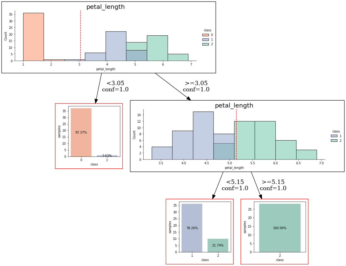
[petal_length  lt 3.05] ==> [class set 0]. # 0.9579256691362875
xrule tree/1:
[petal_length  gte 3.05, petal_length  lt 5.15] ==> [class set 1]. # 0.8398308552545226
xrule tree/2:
[petal_length  gte 3.05, petal_length  gte 5.15] ==> [class set 2]. # 0.9833409059468439
Similarly you can obtain visualization of the rule-based model in a form of decision tree by executing following code.
import graphviz
from graphviz import Source
from IPython.display import SVG, Image
lux.uid3.tree.save_dot('tree.dot',fmt='.2f',visual=True, background_data=train)
gvz=graphviz.Source.from_file('tree.dot')
!dot -Tpng tree.dot > tree.png
Image('tree.png')
The code should yield something like that (depending on the instance that was selected):
The software is the direct implementation of a method described in the following paper:
@misc{bobek2023local,
      title={Local Universal Explainer ({LUX}) -- a rule-based explainer with factual, counterfactual and visual explanations},
      author={Szymon Bobek and Grzegorz J. Nalepa},
      year={2023},
      eprint={2310.14894},
      archivePrefix={arXiv},
      primaryClass={cs.AI}

}


