
The code I used for doing this project can be found in project04.py and Project04.ipynb. All the line numbers I refer to in this document is for project04.py. The following sections go into further detail about the specific points described in the Rubric.
Project 04 - Advanced Lane Detection

Usage:
  project04.py <input_video> <output_video> [-c <camera_file>]
  project04.py (-h | --help)

Options:
  -h --help         Show this screen.
  -c <camera_file>  Specify camera calibration file [default: camera_data.npz]
To run the program with default settings on a video:
python project04.py input_video.mp4 output/output_video.mp4
The camera calibration data gets saved into camera_data.npz by default and is reused in subsequent runs. If you want to change the camera information, delete the file, or specify a different filename using the -c command line argument.
The camera calibration code is contained in lines 25-50 in the functions calibrate_camera and camera_setup. The camera calibration information is cached using numpy.savez_compressed in the interest of saving time. The calibration is performed using chessboard pattern images taken using the same camera as the project videos, such as the one shown below:

The chessboard pattern calibration images (in the cal_images folder) contain 9 and 6 corners in the horizontal and vertical directions, respectively (as shown above). First, a list of "object points", which are the (x, y, z) coordinates of these chessboard corners in the real-world in 3D space, is compiled. The chessboard is assumed to be in the plane z=0, with the top-left corner at the origin. There is assumed to be unit spacing between the corners. These coordinates are stored in the array objp.
  # cal_images contains names of calibration image files
  for fname in cal_images:
      img = cv2.imread(fname)
      gray = cv2.cvtColor(img, cv2.COLOR_BGR2GRAY)

      ret, corners = cv2.findChessboardCorners(gray, (nx, ny), None)
      if ret == True:
          objpoints.append(objp)
          imgpoints.append(corners)

  ret, cam_mtx, cam_dist, rvecs, tvecs = cv2.calibrateCamera(objpoints, imgpoints, gray.shape[::-1],None,None)
For each calibration image, the image coordinates (x,y), of the chessboard corners are computed using the cv2.findChessboardCorners function. These are appended to the imgpoints array and the objp array is appended to the objpoints array.
The two accumulated lists, imgpoints and objpoints are then passed into cv2.calibrateCamera to obtain the camera calibration and distortion coefficients as shown in the above code block. The input image is then undistorted (later in the image processing pipeline on line 409) using these coefficients and the cv2.undistort function.
The image from the camera is undistorted using the camera calibration matrix and distortion coefficients computed in the previous step. This is done using the cv2.undistort function as shown below:
undist = cv2.undistort(image, cam_mtx, cam_dist, None, cam_mtx)
An example of an image before and after the distortion correction procedure is shown below.

Initially a number of combinations of color and gradient thresholds were attempted. It was found that none of these were very robust to changing conditions in lighting and contrast. After reviewing some literature on the subject, it was found that using a second derivative operation (Laplacian) might be more suited to this purpose[1]. By using a Laplacian filter (using cv2.Laplacian) on the image followed by thresholding it to highlight only the negative values (denoting a dark-bright-dark edge) it was possible to reject many of the false positives [ Ref ]. The Laplacian resulted in better results than using combinations of Sobel gradients.
The thresholding operations used to detect edges in the images can be found in lines 149-170 of project_04.py in the function called find_edges. The thresholded binary mask obtained from the Laplacian is named mask_one in the code. The thresholding is first performed on the S-channel of the image in HLS colorspace. If too few pixels were detected by this method (less than 1% of total number of pixels), then the Laplacian thresholding is attempted on the grayscale image.
The second thresholded mask, mask_two, is created using a simple threshold on the S-channel. And finally, a brightness mask (gray_binary) is used to reject any darker lines in the final result. These masks are combined as:
combined_mask = gray_binary AND (mask_one OR mask_two)
The results obtained using the edge detection algorithm for an image is shown below:

The perspective transformation is computed using the functions find_perspective_points and get_perspective_transform in lines 52-147 of project04.py. find_perspective_points uses the method from [project1][Project 1] to detect lane lines. Since the lanes are approximated as lines, it can be used to extract four points that are actually on the road which can then be used as the "source" points for a perspective transform.
Here is a brief description of how ths works:
- Perform thresholding/edge detection on the input image
- Mask out the upper 60% of pixels to remove any distracting features
- Use Hough transforms to detect the left and right lane markers
- Find the apex-point where the two lines intersect. Choose a point a little below that point to form a trapezoid with four points -- two base points of lane markers + upper points of trapezoid
- Pass these points along with a hardcoded set of destination points to
cv2.getPerspectiveTransformto compute the perspective transformation matrix
Note: In case the hough transform fails to detect the lane markers, a hardcoded set of source points are used
The original and warped images along with the source points (computed dynamically) and destination points used to computed the perspective transform, are shown below:

The lane detection was primarily performed using two methods -- histogram method and masking method. The latter only works when we have some prior knowledge about the location of the lane lines. A sanity check based on the radius of curvature of the lanes is used to assess the results of lane detection. If two many frames fail the sanity check, the algorithm reverts to the histogram method until the lane is detected again.
Both methods also use a sanity check which checks if the radius of curvature of the lanes have changed too much from the previous frame. If the sanity check fails, the frame is considered to be a "dropped frame" and the previously calculated lane curve is used. If more than 16 dropped frames are consecutively encountered, the algorithm switches back to the histogram method.
The first step in this method is to compute the base points of the lanes. This is done in the histogram_base_points function in lines 352-366 of project04.py. The first step is to compute a histogram of the lower half of the thresholded image. The histogram corresponding to the thresholded, warped image in the previous section is shown below:

The find_peaks_cwt function from the scipy.signal is used to identify the peaks in the histogram. The indices thus obtained are further filtered to reject any below a certain minimum value as well as any peaks very close to the edges of the image. For the histogram shown above, the base points for the lanes are found to be at the points 297 and 1000.
Once the base points are found, a sliding window method is used to extract the lane pixels. This can be seen in the sliding_window function in lines 308-346. The algorithm splits the image into a number of horizontal bands (10 by default). Starting at the lowest band, a window of a fixed width (20% of image width) centered at both base points is considered. The x and y coordinates of all the nonzero pixels in these windows are compiled into into separate lists. The base point for the next band is assumed to be the column with the maximum number of pixels in the current band. After all the points are accumulated, the function reject_outliers is used to remove any points whose x or y coordinates are outside of two standard deviations from the mean value. This helps remove irrelevant pixels from the data.
The filtered pixels are then passed into the add_lane_pixels method of the Lane class defined in lines 200-248. These pixels, along with a weighted average of prior lane pixels are used with np.polyfit to compute a second order polynomial that fits the points.
The polynomial is then used to create an image mask that describes a region of interest which is then used by the masking method in upcoming frames.

This is the less computationally expensive procedure that is used when a lane has already been detected before. The previously detected lanes are used to define regions of interest where the lanes are likely to be in (shown in image above). This is implemented in the detect_from_mask method defined in lines 276-283. The algorithm uses the mask generated during the histogram method to remove irrelevant pixels and then uses all non-zero pixels found in the region of interest with the add_lane_pixels method to compute the polynomial describing the lane.
The sanity check is defined in the method sanity_check_lane in lines 259-269. It is called by the add_lane_pixels method regardless of what method is used to detect the lane pixels. The stored value of the radius of curvature of the lane is used to see if the current radius of curvature has deviated by more than 50% in which case.
  R0 = self.radius_of_curvature
  self.insanity = abs(R-R0)/R0  # R = current radius of curvature
return self.insanity <= 0.5The radius of curvature is computed in the compute_rad_curv method of the Lane class in lines 251-257. The pixel values of the lane are scaled into meters using the scaling factors defined as follows:
ym_per_pix = 30/720 # meters per pixel in y dimension
xm_per_pix = 3.7/700 # meteres per pixel in x dimension
These values are then used to compute the polynomial coefficients in meters and then the formula given in the lectures is used to compute the radius of curvature.
The position of the vehicle is computed by the code in lines 455-456. The camera is assumed to be centered in the vehicle and checks how far the midpoint of the two lanes is from the center of the image.
middle = (left_fitx[-1] + right_fitx[-1])//2
veh_pos = image.shape[1]//2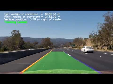
dx = (veh_pos - middle)*xm_per_pix # Positive on right, Negative on leftThe complete pipeline is defined in the process_image function in lines 355-475 that performs all these steps and then draws the lanes as well as the radius and position information on to the frame. The steps in the algorithm are:
Distortion correction → Edge Detection → Perspective Transform → Lane Detection (using Histogram or Masking methods) → Sanity Check
An example image that was run through the pipeline is shown below:

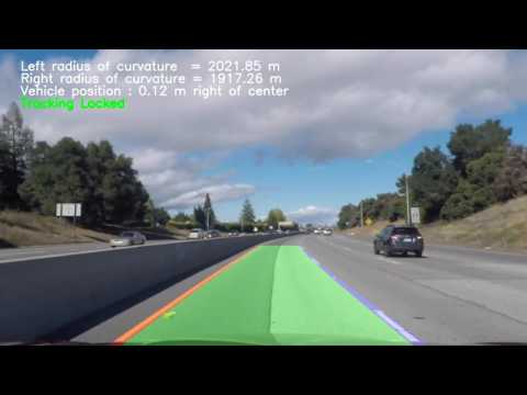
Project video output
This same video can also be found at: project_video_out.mp4
Challenge video output
The lanes in the harder challenge video were found to be very difficult to track with this pipeline. The algorithm has to be improved and made more robust for that video.
The pipeline was able to detect and track the lanes reliably in the project video. With some tweaks (reversing the warping/edge detection), it also worked well for the challenge video. The main issue with the challenge video was lack of contrast and false lines.
A color image can be converted to grayscale in many ways. The easiest is what is called equal-weight conversion where the red, green and blue values are given equal weights and averaged. However, the ratio between these weights can be modified to enhance the gradient of the edges of interest (such as lanes). According to Ref.2, grayscale images converted using the ratios 0.5 for red, 0.4 for green, and 0.1 for blue, are better at detecting yellow and white lanes. This method was used for converting images to gray scale in this project.
However, even this method faces problems under different color temperature illuminations, such as evening sun or artificial lighting conditions. A better method that continuously computes the best weighting vector based on prior frames is described in [2]. This was not implemented in this project due to time constraints, and because reasonable results were obtained for the project and challenge videos without the use of such a method. However, implementing such a method would make the pipeline a lot more robust to change in contrast and illumination.
In the pipeline described in the lectures, the perspective transform was applied after the edges were detected in the image using some thresholding techniques (described in a later section).
The effect of reversing this order, by applying the perspective transform first and then applying the edge detection was also examined. It was found that with the current set of hyper-parameters used for edge detection, the reverse process was able to reject more "distractions" at the cost of a decrease in the number of lane pixels found. This was particularly of interest in some parts of the challenge video. Here is an example of an image where the order of thresholding and warping made a difference:

However, the effect wasn't significant enough to merit its use in the final version. The reversed order of operations was also found to remove too many legitimate lane pixels. challenge_video_out2.mp4 is an example of video output using the reverse order of operations. This option can be enabled by commenting the lines 392-393 and uncommenting lines 396-397. This hack is probably not needed with a better gradient enhancement process.
Steerable filters[3] are convolution kernels that can detect edges oriented at certain angles. This might especially be useful in cases like the harder challenge video where the lane line is practically horizontal in some frames.
Euler spirals, also known as clothoids, are parametric curves whose curvature changes linearly with the independent variable. They are frequently used in highway engineering to design connecting roads, on and off ramps etc. These might be a better candidate curve to fit to the lane pixels rather than simple second order polynomials.
[1] Juneja, M., & Sandhu, P. S. (2009). Performance evaluation of edge detection techniques for images in spatial domain. International Journal of Computer Theory and Engineering, 1(5), 614.
[2] Yoo, H., Yang, U., & Sohn, K. (2013). Gradient-enhancing conversion for illumination-robust lane detection. IEEE Transactions on Intelligent Transportation Systems, 14(3), 1083-1094.
[3] McCall, J. C., & Trivedi, M. M. (2006). Video-based lane estimation and tracking for driver assistance: survey, system, and evaluation. IEEE transactions on intelligent transportation systems, 7(1), 20-37.