Quanvolutional Neural Network (QNN)

In this notebook we implement a Quanvolutional Neural Network, a quantum machine learning model originally introduced in Henderson et al. (2019).

CNN vs. QNN

A Convolutional Neural Network (CNN) is a standard model in (classical) machine learning, especially suitable for image processing. This model is based on the idea of a convolution layer where, instead of processing the full input data with a global function, a local convolution is applied. Small local regions are sequentially processed with the same kernel. The results obtained for each region are then associated to different channels of a single output pixel. The union of all the output pixels produces a new image-like object, which can be further processed by additional layers.

One can then consider quantum variational circuits, which are quantum algorithms depending on free parameters. These algorithms are trained by a classical optimization algorithm that makes queries to the quantum device, the optimization being an iterative scheme that searches out better candidates for the parameters with every step. Variational circuits have become popular as a way to think about quantum algorithms for near-term quantum devices.

In this project we implement a simplified approach, which still allows us to grasp the idea behind the so-called Quanvolutional Neural Networks (QNNs). The scheme is represented in the figure.

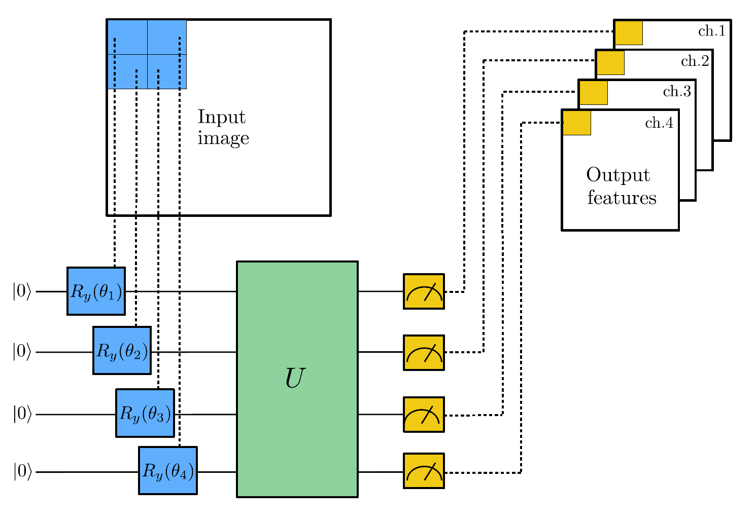
1. A small region of the input image, in our example a 2×2 square, is embedded into a quantum circuit – this is achieved with parametrized rotations applied to the qubits initialized in the ground state.
2. A quantum computation, associated to a unitary U, is performed on the system – the unitary could be generated by a variational quantum circuit or, more simply, by a random circuit as proposed in Henderson et al. (2019).
3. The quantum system is measured, obtaining a list of classical expectation values.
4. Analogously to a classical convolution layer, each expectation value is mapped to a different channel of a single output pixel.
5. Iterating the same procedure over different regions, one can scan the full input image, producing an output object which will be structured as a multi-channel image.

Note that:

• a fixed non-trainable quantum circuit is used as a quanvolution kernel, while the subsequent classical layers are trained for the classification purpose;
• the quanvolution can be followed by further quantum layers or by classical layers;
• the main difference with respect to a classical convolution is that a quantum circuit can generate highly-complex kernels whose computation could be – at least in principle – classically intractable.

Quanvolution layer

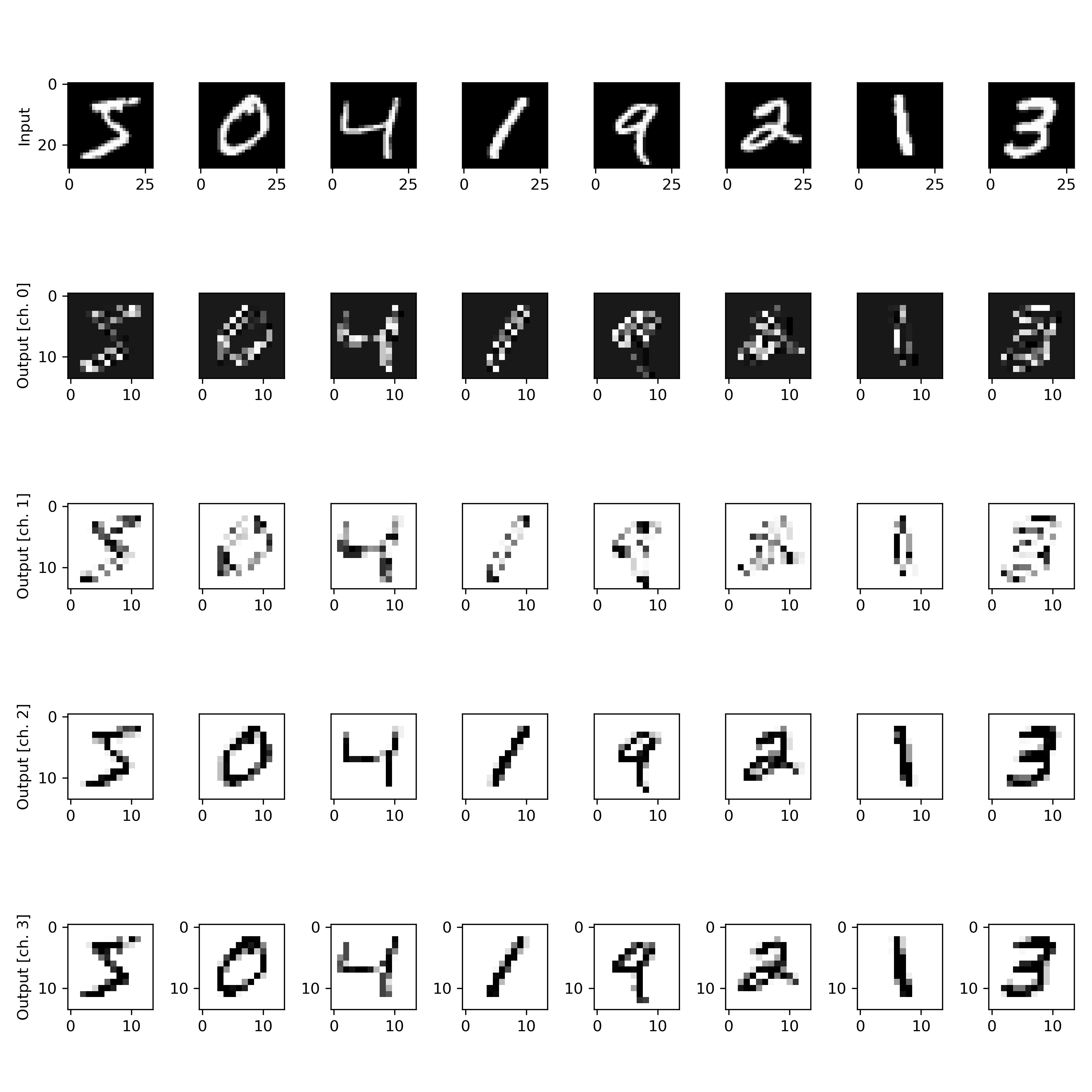
The effect of the quantum convolution layer can be visualised on a batch of samples: below each input image, the 4 output channels generated by the quanvolution are shown.

CNN vs. QNN – Accuracy

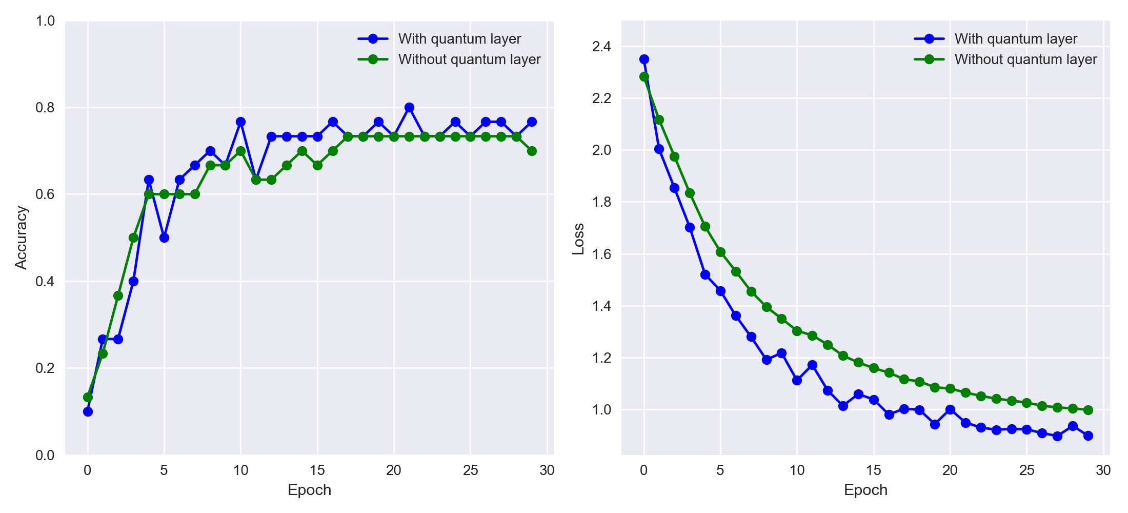
We deploy this "toy" model on the MNIST (handwritten digits) dataset, where it seems that QNNs can achieve both higher accuracy and faster training compared to a purely classical CNN – as pointed out in Henderson et al. (2019).