CNN-coreflooding-muCT

Segment core-flooding micro-CT images using CNN.

This work uses the U-Net architecture implemented by : https://github.com/jvanvugt/pytorch-unet

Training template and example using ipython notebook: https://yclipse.github.io/CNN-core-flooding-muCT/

The trained model can be downloaded via : https://drive.google.com/file/d/18-Gna1Xr8JFSIsWGmflSBow3VkO8tS1B/view?usp=sharing

Tutorial for muCT image processing and segmentation using scikit-image please visit : https://github.com/yclipse/muCTimage_processing_tutorial

Prerequisite

PyTorch

CUDA toolkit (enable GPU acceleration)

Example CNN architecture

Training template and example

This document is a training code template that only used 10 training images and trained for 50 epochs for tutorial purpose.

Users can test this code using the training images from https://github.com/yclipse/CNN-core-flooding-muCT.

Users can use their own dataset to train a CNN segmentation model for CT images, add customised functions and fine-tune the parameters for the best result.

Import modules

%matplotlib inline
#import from installed python libraries
import torch
import os
import os.path
import torch.nn as nn
import torch.nn.functional as F
import matplotlib.pyplot as plt
import numpy as np
import glob
from PIL import Image
# import sys
# from joblib import Parallel, delayed
# import time
# import scipy.misc
print ('modules imported')

#import from local ipynb file
from ipynb.fs.full.function_kits import test_availability,im2array,imview,im_compare,rescale
from .defs.Unet import UNet

test_availability()
print (torch.cuda.is_available())
print ('torch Ver .', torch.__version__)

modules imported
toolbox functions available
toolbox functions available
True
torch Ver . 1.0.0

Import the CT image files, and their corresponding ground truth images

img_dir='N:/CNN_SEG/figures/example/img/'
gt_dir='N:/CNN_SEG/figures/example/gt'
img_list=sorted(glob.glob(os.path.join(img_dir,'*.tif')))
gt_list=sorted(glob.glob(os.path.join(gt_dir,'*.tif')))

Split the images into a training dataset, a validation dataset and a test dataset. Here I produced a 80%: 10%: 10% split. And pair each image with its corresponding ground truth.

train_set=(img_list[:8],gt_list[:8])
val_set=(img_list[8:9],gt_list[8:9])
test_set=(img_list[-1:],gt_list[-1:])

The following two functions convert each image file into 'tensor' that is a multi-dimensional matrix containing elements of a single data type. It is basically the pytorch version of numpy array. The images are down-sampled (2x2 mean pooling) and cropped into a suitable size for the GPU. You need to adjust the code to fit the size of your own data and GPU.

from skimage.measure import block_reduce
def img2tensor(file,unsqueeze=False):
    img=Image.open(file)
    ####################################################change this block according to your own data size and make some pre-processing
    imarray=np.asarray(img)[110:1582,100:1572]
    downsample=block_reduce(imarray, block_size=(2,2), func=np.mean)[120:616,120:616]
    imarray_rescale=rescale(downsample)
    imtensor = torch.from_numpy(imarray_rescale).type(torch.float)
    ####################################################change this block according to your own data size and make some pre-processing
    if unsqueeze==True:
        imtensor =  torch.unsqueeze(imtensor, dim=0)
    return imtensor
def label2tensor(file):
    img=Image.open(file)
    ####################################################change this block according to your own data size and make some pre-processing
    imarray=np.asarray(img)[110:1582,100:1572]
    downsample=block_reduce(imarray, block_size=(2,2), func=np.mean)[120:616,120:616]
    labels=np.zeros(downsample.shape)
    labels[downsample==0]=0#bg       #the groundtruth image is labelled with 0-127-255 for three classes, here I converted them to 1-2-3
    labels[downsample==127]=1#oil
    labels[downsample==255]=2#brine
    ####################################################change this block according to your own data size and make some pre-processing
    imtensor = torch.from_numpy(labels).type(torch.float)
    return imtensor

Define the Data_imoprter function to import the dataset into the CNN model when initialising training

from torch.utils.data import Dataset, DataLoader
class Data_importer(Dataset):
    """
    A customized data loader.|
    """
    def __init__(self, datalist,labellist):
        """ Intialize the dataset
        """
        self.x_data=datalist
        self.y_data=labellist
        self.len = len(datalist)
        
    # You must override __getitem__ and __len__
    def __getitem__(self, index):
        """ Get a sample from the dataset
        """
        traintensor= img2tensor(self.x_data[index],unsqueeze=True)
        labeltensor= label2tensor(self.y_data[index])
        #
        return traintensor,labeltensor.long()

    def __len__(self):
        """
        Total number of samples in the dataset
        """
        return self.len

Define some Evaluation functions

Receiver operating characteristic (ROC)

ROC curve is a graphical plot that illustrates the diagnostic ability of a binary classifier system as its discrimination threshold is varied.

The ROC curve is created by plotting the true positive rate (TPR) against the false positive rate (FPR) at various threshold settings. The true-positive rate is also known as sensitivity, recall or probability of detection in machine learning

TP = True positive; FP = False positive; TN = True negative; FN = False negative

precision, recall, accuracy and F1 score

precision: tp / (tp + fp) => how many selected items are relevant?

recall: tp / (tp + fn) => how many relevant items are selected?

F1: harmonic mean of precision and recall

accuracy:(tp + tn) / (tp + tn + fp + fn) => the proportion of true results (both true positives and true negatives) among the total number of cases examined

Intersection over Union (IOU)

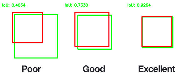
Intersection :area of overlap between the predicted area and the ground-truth area

Union: the area encompassed by both the predicted area and the ground-truth area.

IOU = Intersection/Union

def eval_metrics(pred,gt):
    tp=((pred == 1) & (gt == 1)).sum()
    # TN    predict 0 label 0
    tn=((pred == 0) & (gt == 0)).sum()
    # FN    predict 0 label 1
    fn=((pred == 0) & (gt == 1)).sum()
    # FP    predict 1 label 0
    fp=((pred == 1) & (gt == 0)).sum()
#   precision=tp/ (tp + fp)
#   recall = tp/ (tp + fn)
#   F1 = 2 * (recall*precision) / (recall+precision)
    rand = (tp + tn) / (tp + tn + fp + fn)  #rand index
    iou = tp / (tp + fp + fn)   #Intersection over Union
    return rand, iou

The CNN model output is a prediction of scores of each pixel belonging to a class. We use the softmax function to convert the scores into probabilities that are values between 0 and 1, and the three classes add up to 1. We classify the pixels with the largest probability of each class. This function below essentially convert the CNN prediction into segmentation labels.

def prob_to_labels(prediction):
    m = nn.Softmax2d() 
    prob=m(prediction)
    seg_labels=np.zeros(prob.cpu().detach().numpy()[0][0].shape)
    rock=prob.cpu().detach().numpy()[0][0]
    oil=prob.cpu().detach().numpy()[0][1]
    brine=prob.cpu().detach().numpy()[0][2]
    seg_labels[rock-oil-brine>0]=0
    seg_labels[oil-rock-brine>0]=1
    seg_labels[brine-oil-rock>0]=2
    return seg_labels

These two functions below will produce the rand index of each phase and the mean IoU as measurements of segmentation quality

import statistics
def threephase_accuracy(phase,seg_labels,gt):
    p={'rock':0,'oil':1,'brine':2}
    rand,iou=eval_metrics(seg_labels==p[phase],gt==p[phase])
    return rand,iou
def measure_accuracy(prediction,y):
    seg_labels=prob_to_labels(prediction)
    gt=y.cpu().detach().numpy()[0] 
    rand_rock,iou_rock=threephase_accuracy(phase='rock',seg_labels=seg_labels,gt=gt)
    rand_oil,iou_oil=threephase_accuracy(phase='oil',seg_labels=seg_labels,gt=gt)
    rand_brine,iou_brine=threephase_accuracy(phase='brine',seg_labels=seg_labels,gt=gt)
    mean_accuracy=statistics.mean([rand_rock,rand_oil,rand_brine])
    mean_iou=statistics.mean([iou_rock,iou_oil,iou_brine])
    return  rand_rock,rand_oil,rand_brine,mean_iou

Initialise training, load the data using the Data_importer and DataLoader functions.

train_dataset=Data_importer(train_set[0],train_set[1])
train_loader=DataLoader(train_dataset,
                        batch_size=1,
                        shuffle=False,
                        num_workers=0
                       )

val_dataset=Data_importer(val_set[0],val_set[1])
val_loader=DataLoader(val_dataset,
                        batch_size=1,
                        shuffle=False,
                        num_workers=0
                       )

Hyperparameters are pre-defined parameters that controls the overall learning behaviour of the CNN model

Epoch and mini-batch

Use multiple epochs to train the same dataset multiple times. (often use shuffle to change traning sequence to get better resutls.)
Use batch_size to slice data into mini-batches

Learning rate

Learning rate controls the step size of learning.

Batch normalisation L2

Use batch normalisation to make activation funtion more sensitive

Optimizer

make training faster
adam > RMSprop > Momentum > SGD

EPOCHS = 50          # Use multiple epochs to train the same dataset multiple times. 
BATCH_SIZE = 1            #Use batch_size to slice data into mini-batches
LR = 5e-5              # learning rate try  1e-4 later
L2_penalty=1e-5        #add a L2 penalty (regulisation) to alleviate over-fitting

We use CUDA to enable GPU acceleration, import the U-Net model, and apply an Adam optimizer

device = torch.device('cuda' if torch.cuda.is_available() else 'cpu')
model = UNet(in_channels=1, n_classes=3, depth=5, wf=6, padding=True,
                 batch_norm=True, up_mode='upconv').to(device)     #batch normalisation: To increase the stability of a neural network
optim = torch.optim.Adam(model.parameters(),lr=LR, weight_decay=L2_penalty)  # accelerate gradient descent using Adam

Define some empty list to record the training loss and accuracy during training

dic=["rand_rock","rand_oil","rand_brine",'mean_iou']
eval_dic={}
ave_acc={}
train_loss_rec=[]
val_loss_rec=[]
train_loss_ave=[]
val_loss_ave=[]
for i in range(len(dic)):
    eval_dic[dic[i]]=[]
    ave_acc[dic[i]]=[]

def ave_list(lst):
    return sum(lst)/len(lst)

Start training

Validation at the end of each training epoch. You can also do validation for every n epochs if you have many training epochs. The loss scores and accuracy measurements are printed every epoch to track the training process.

print('start training')    

for epoch in range(EPOCHS):
        ###################
        # train the model #
        ###################
    model.train()

    for iteration, (x,y) in enumerate(train_loader):
        x=x.to(device)
        y=y.to(device)
        x =  torch.autograd.Variable(x)
        y =  torch.autograd.Variable(y)
        prediction = model(x)  # [N, 2, H, W]
        #get loss
        loss = F.cross_entropy(prediction, y)
        train_loss_rec.append(loss.data.cpu().detach().numpy())
        optim.zero_grad()
        loss.backward()
        optim.step()
        sys.stdout.write('\r epoch {}  training {} steps  train loss: {}'.format(epoch, iteration+1,loss.data.cpu().detach().numpy())) #print text progress
        sys.stdout.flush()
        
    print ('\r saving model..')
    torch.save(model.state_dict(), 'N:\\CNN_SEG\\CODES\\Unet_example_epoch{}.pth'.format(epoch)) 
    
        ######################    
        # validate the model #
        ######################
         #end of each training epoch
    if epoch%1==0: #every 1 epoch validation 
        #save in every 1 epochs

        print ('\r validating..')
        #epoch_train_loss.append(loss.data.cpu().detach().numpy())
        
        model.eval()
        for i,(val_x,val_y) in enumerate(val_loader):
            val_x=val_x.to(device)
            val_y=val_y.to(device)
            val_x =  torch.autograd.Variable(val_x)
            val_y =  torch.autograd.Variable(val_y)
            val_prediction = model(val_x)  # [N, 2, H, W]
            val_loss = F.cross_entropy(val_prediction, val_y)
            val_loss_rec.append(val_loss.data.cpu().detach().numpy())
            #get accuracy
            tuple_dic=(rand_rock,rand_oil,rand_brine,mean_iou)=measure_accuracy(val_prediction,val_y)
            #print progress 
            sys.stdout.write('\r validating {} steps'.format(i+1)) #print text progress
            sys.stdout.flush()
            for i in range(len(dic)):
                eval_dic[dic[i]].append(tuple_dic[i])
        for i in range(len(dic)):
            ave_acc[dic[i]].append(ave_list(eval_dic[dic[i]]))
        #plot eval accuracy
        fig, axes = plt.subplots(ncols=1,nrows=2)
        fig.set_size_inches(20, 8)
        ax1,ax2=axes
        #validation accuracy
        for i in range(len(dic)):
            ax1.plot(range(len(ave_acc[dic[i]])),ave_acc[dic[i]],'.-',label=dic[i],linewidth=6-i)
        ax1.legend(loc=(1,0.5))  
        #validation loss
        train_loss_ave.append(ave_list(train_loss_rec))
        val_loss_ave.append(ave_list(val_loss_rec))
        ax2.plot(range(epoch+1),train_loss_ave,'.-',label='train_loss')
        ax2.plot(range(epoch+1),val_loss_ave,'.-',label='val_loss')
        ax2.legend()
        plt.savefig('N:/CNN_SEG/figures/example/train_val_history_epoch{}.png'.format(epoch+1), bbox_inches='tight')
        plt.pause(0.05)

validating..aining 8 steps train loss: 0.6303515434265137

Visualise the probability of each class

m=nn.Softmax2d()
prob=m(prediction)
brine=prob.cpu().detach().numpy()[0][2]
oil=prob.cpu().detach().numpy()[0][1]
solid=prob.cpu().detach().numpy()[0][0]

fig, axes = plt.subplots(nrows=1,ncols=3)
ax0, ax1,ax2 = axes

ax0.imshow(solid)
ax0.set_title('Probability Distribution - Solid',fontsize=18)
ax0.axis('off')
ax1.imshow(oil)
ax1.set_title('Probability Distribution - Oil',fontsize=18)
ax1.axis('off')
ax2.imshow(brine)
ax2.set_title('Probability Distribution - Brine',fontsize=18)
ax2.axis('off')       

fig.set_size_inches(20, 14)


cax2 = ax2.imshow(brine, interpolation='nearest', vmin=0, vmax=1,cmap='seismic')
cax1 = ax1.imshow(oil, interpolation='nearest', vmin=0, vmax=1,cmap='seismic')
cax0 = ax0.imshow(solid, interpolation='nearest', vmin=0, vmax=1,cmap='seismic')

cb0 = fig.colorbar(cax0,ax=ax0,shrink=0.4)  
cb1 = fig.colorbar(cax1,ax=ax1,shrink=0.4)
cb2 = fig.colorbar(cax2,ax=ax2,shrink=0.4)  


cb0.ax.set_ylabel('Probability', rotation=90)
cb1.ax.set_ylabel('Probability', rotation=90)
cb2.ax.set_ylabel('Probability', rotation=90)

fig.subplots_adjust(left=None, bottom=None, right=None, top=None, wspace=None, hspace=None)
fig.tight_layout()

Check segmentation image result

def imgresult(x,y,pred):
    raw=x.cpu().detach().numpy()[0][0]
    gt=y.cpu().detach().numpy()[0]
    seg_labels=prob_to_labels(prediction)
    
    fig, axes = plt.subplots(nrows=1,ncols=3)
    ax0, ax1,ax2 = axes

    ax0.imshow(raw,cmap='gray')
    ax0.set_title('Raw Image',fontsize=18)
    ax0.axis('off')
    ax1.imshow(gt,cmap='plasma')
    ax1.set_title('Ground Truth',fontsize=18)
    ax1.axis('off')
    ax2.imshow(seg_labels,cmap='plasma')
    ax2.set_title('CNN Segmentation',fontsize=18)
    ax2.axis('off')       
    fig.set_size_inches(20, 14)
    plt.pause(0.01)
    

imgresult(x,y,prediction)

Testing

model_test = UNet(in_channels=1, n_classes=3, depth=5, wf=6, padding=True,
                 batch_norm=True, up_mode='upconv').to(device)
#model_test.load_state_dict(torch.load('8.pth'))

test_dataset=Data_importer(test_set[0],test_set[1])
test_loader=DataLoader(test_dataset,
                        batch_size=BATCH_SIZE,
                        shuffle=True,
                        num_workers=0
                       )

test_dic={}
test_ave_acc={}
for i in range(len(dic)):
    test_dic[dic[i]]=[]
    test_ave_acc[dic[i]]=[]

print('start testing')
model_test.eval()
for i,(test_x,test_y) in enumerate(test_loader):
    test_x=test_x.to(device)
    test_y=test_y.to(device)
    test_x =  torch.autograd.Variable(test_x)
    test_y =  torch.autograd.Variable(test_y)
    test_prediction = model_test(test_x)  # [N, 2, H, W]
    
    #get accuracy
    tuple_dic=(rand_rock,rand_oil,rand_brine,mean_iou)=measure_accuracy(test_prediction,test_y)

    for i in range(len(dic)):
        test_dic[dic[i]].append(tuple_dic[i]) 


for i in range(len(dic)):
    test_ave_acc[dic[i]].append(ave_list(test_dic[dic[i]]))
#print test accuracy
print(test_ave_acc)

start testing
{'rand_rock': [0.943792273673257], 'rand_oil': [0.9619252406347555], 'rand_brine': [0.9818670330385015], 'mean_iou': [0.31459742455775236]}