bedtorch

For full documentation, refer to the package documentation site.

Motivation

The goal of bedtorch is to provide a fast BED file manipulation tool suite native in R.

In bioinformatics studies, an important type of jobs is related to BED and BED-like file manipulation. To name a few example:

• Filtering cfDNA fragments based on length
• Identifying genomic regions overlapping with certain genes
• Filtering features based on epigenetic profiles such as histone modification levels
• Extracting SNVs in a certain genomic interval

Many of such tasks can be done by some highly-optimized tools, such as bedtools and bedops. However, these are binary tools which only works in shell. Sometimes, especially for developers using R, it’s desirable to invoke these tools in R codes.

One solution is using functions that invokes system commands (system2 or system). bedr, a popular package, is one good example. It’s a bridge linking between R codes and shell tools. Under the hood, it writes data into the temporary directory, calls certain command line tools such as tabix, bedtools, or bedops, parses the output and re-generate a data frame in R space.

Generally this approach is very helpful. However, it’s worth noting some disadvantages.

• This workflow requires lots of disk IO, since data frames in R needs to be written to temporary directories before being fed to command line tools.
• Command line output is captured and transferred back to R s space. The data transfer is done by stdin/stdout pipes. For R, reading large amount of text content from stdin can be extremely slow. As a result, most of time when large dataset is involved, bedr is hardly usable.
• bedr captures command line output as plain text. Therefore, when the data is transferred back to R, most of the information about data types, index (in the case of data.table), column names, etc., are lost. It’s the package user’s responsibility to make sure data types are correct, column names are restored, column indices have been rebuilt (in the case of data.table, which can be very time consuming). Often this job is tedious, error-prone and introduces very large overheads.
• It requires the command line tools to be present in PATH. This depends on the end user’s system environment and the R developer can do nothing about it. It puts additional burden to deployment, especially when the end user is not an IT professional.

Another approach is using native R data types to represent BED-like data. R’s native data.frame seems to be a good model, but in many scenarios, it’s performance is poor. More importantly, it lacks many advanced features compared with GenomicRanges, dplyr and data.table.

GenomicRanges is widely used in bioinformatics community. Although it provides essential building blocks for many tasks, such as findOverlaps, reduce, etc., it doesn’t provide high-level features as bedtools does. Using findOverlaps, reduce, and other functions provided by GenomicRanges, users may implement operations such as map, merge, unique intersect, but this still requires lots of coding.

It would be desirable to have an R package, which represent BED-like data by GenomicRanges or data.table objects, and provide native support for common BED manipulations, such as merge, intersect, filter, etc.

Details

bedtorch is an attempt for this. Under the hood, every BED dataset is represented as a GenomicRanges object (it also can represent the dataset as data.table, if preferred. But this is not recommended). Users can apply various operations on it, such as intersect, merge, etc.

In terms of the core computation, bedtorch’s performance is comparable to bedtools. However, since no disk IO and data conversion is needed, users can directly manipulate the dataset in memory, therefore in practice, via bedtorch, many tasks can be done about one magnitude faster.

Additionally, by linking to htslib, bedtorch can write data frames directly to BGZIP-format files, and optionally create the tabix index. It can also directly load either local or remote BGZIP-format files at any particular genomic regions. This feature is done by htslib, therefore not requiring external command line tools such as tabix or bgzip. In the case of working with remote files, being capable of loading any arbitrary portion of the file will be very convenient.

BGZIP is a variant of gzip and is widely used in bioinformatics. It’s compatible with gzip, with an important additional feature: allows a compressed file to be indexed for fast query. However, R is unaware of BGZIP. It considers all .gz files as gzip-compressed, thus doesn’t take advantage of BED index, and cannot output BGZIP files.

For more details, refer to the package reference page.

Installation

# install.packages("devtools")
devtools::install_github("haizi-zh/bedtorch")

Example

Here are several basic examples which shows you how to solve a common problem:

Read a BED file from disk:

library(bedtorch)

## Load BED data
file_path <-
  system.file("extdata", "example2.bed.gz", package = "bedtorch")

bedtbl <- read_bed(file_path, range = "1:3001-4000")
bedtbl
#> GRanges object with 14 ranges and 2 metadata columns:
#>        seqnames    ranges strand |    score1    score2
#>           <Rle> <IRanges>  <Rle> | <integer> <integer>
#>    [1]        1 2926-3011      * |       106       181
#>    [2]        1 3004-3092      * |        88       193
#>    [3]        1 3092-3193      * |       118       212
#>    [4]        1 3165-3248      * |        94       211
#>    [5]        1 3233-3345      * |       107       205
#>    ...      ...       ...    ... .       ...       ...
#>   [10]        1 3619-3726      * |       108       172
#>   [11]        1 3695-3803      * |       117       214
#>   [12]        1 3777-3867      * |       109       195
#>   [13]        1 3845-3939      * |        92       199
#>   [14]        1 3925-4016      * |        93       197
#>   -------
#>   seqinfo: 1 sequence from an unspecified genome; no seqlengths

Read a remote BGZIP BED file for a certain region:

# Load remote BGZIP files with tabix index specified
# Here we need to explicitly indicate `compression` as `bgzip` since we are
# using short URL for `tabix_index`, so that the function cannot guess
# compression type using the URL
read_bed(
  "https://git.io/JYATB",
  range = "22:20000001-30000001",
  tabix_index = "https://git.io/JYAkT",
  compression = "bgzip"
)
#> GRanges object with 21 ranges and 2 metadata columns:
#>        seqnames            ranges strand |      score comp_method
#>           <Rle>         <IRanges>  <Rle> |  <numeric> <character>
#>    [1]       22 20000001-20500000      * | -0.0613535    cofrag/3
#>    [2]       22 20500001-21000000      * | -0.0422752    cofrag/3
#>    [3]       22 21000001-21500000      * |  0.0268175    cofrag/3
#>    [4]       22 21500001-22000000      * |  0.0386308    cofrag/3
#>    [5]       22 22000001-22500000      * |  0.0265141    cofrag/3
#>    ...      ...               ...    ... .        ...         ...
#>   [17]       22 28000001-28500000      * | 0.08472735    cofrag/3
#>   [18]       22 28500001-29000000      * | 0.15800267    cofrag/3
#>   [19]       22 29000001-29500000      * | 0.14646452    cofrag/3
#>   [20]       22 29500001-30000000      * | 0.07898761    cofrag/3
#>   [21]       22 30000001-30500000      * | 0.00434186    cofrag/3
#>   -------
#>   seqinfo: 1 sequence from an unspecified genome; no seqlengths

Write the previous data table to the temporary directory, and create the tabix index alongside:

write_bed(bedtbl,
          file_path = tempfile(fileext = ".bed.gz"),
          tabix_index = TRUE)

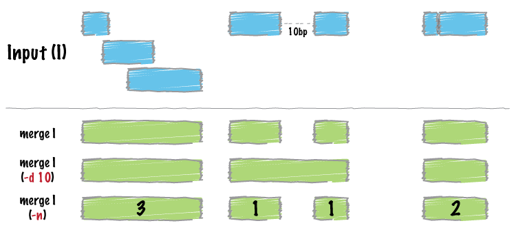
Merge intervals, and take the mean of score in each merged group:

Image by bedtools

operation = list(mean_score = list(on = "score1", func = mean))
merged <- merge_bed(bedtbl, operation = operation)
head(merged)
#> GRanges object with 1 range and 1 metadata column:
#>       seqnames    ranges strand | mean_score
#>          <Rle> <IRanges>  <Rle> |  <numeric>
#>   [1]        1 2926-4016      * |    99.0714
#>   -------
#>   seqinfo: 1 sequence from an unspecified genome; no seqlengths

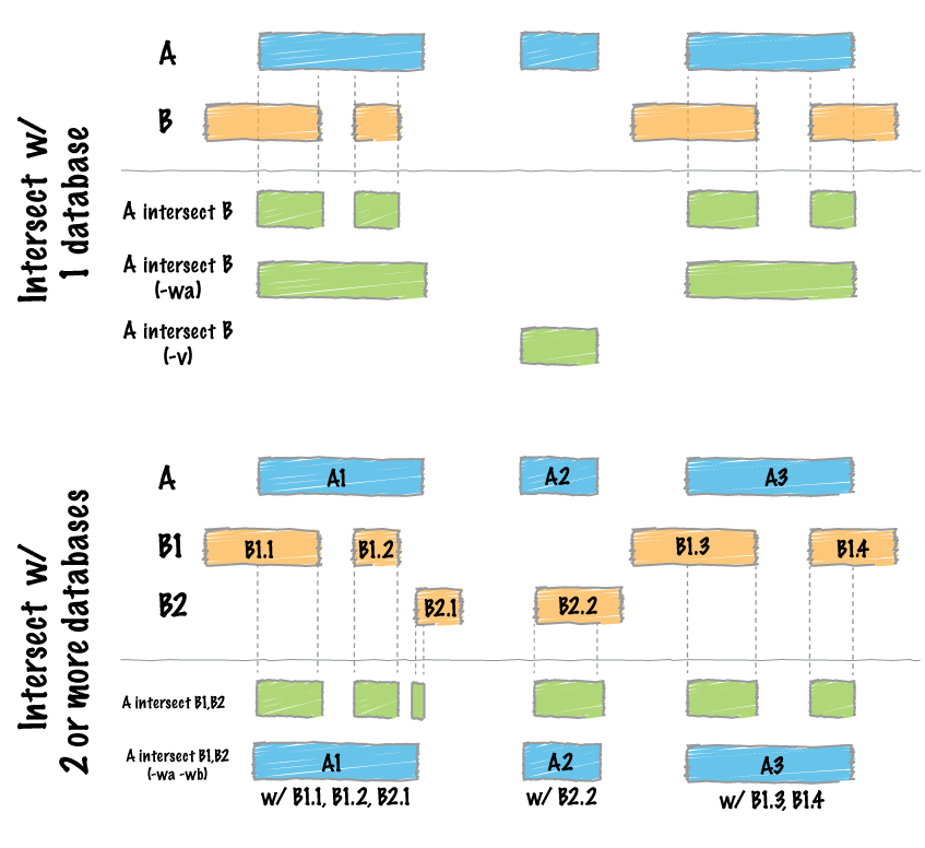
Find intersections between two datasets:

Image by bedtools

file_path1 <- system.file("extdata", "example_merge.bed", package = "bedtorch")
file_path2 <- system.file("extdata", "example_intersect_y.bed", package = "bedtorch")

tbl_x <- read_bed(file_path1, genome = "hs37-1kg")
tbl_y <- read_bed(file_path2, genome = "hs37-1kg")
intersect_bed(tbl_x, tbl_y)
#> GRanges object with 12 ranges and 1 metadata column:
#>        seqnames    ranges strand |     score
#>           <Rle> <IRanges>  <Rle> | <integer>
#>    [1]       21     23-25      * |         7
#>    [2]       21     27-30      * |         7
#>    [3]       21     30-35      * |         9
#>    [4]       21     48-49      * |         1
#>    [5]       21     48-50      * |         2
#>    ...      ...       ...    ... .       ...
#>    [8]       22     43-44      * |         9
#>    [9]       22     47-50      * |         0
#>   [10]       22     52-59      * |         9
#>   [11]       22     54-57      * |         5
#>   [12]       22     58-60      * |         9
#>   -------
#>   seqinfo: 84 sequences from hs37-1kg genome

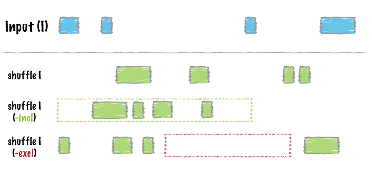
Shuffle a BED data table across the genome:

Image by bedtools

shuffle_bed(tbl_x)
#> GRanges object with 20 ranges and 1 metadata column:
#>        seqnames            ranges strand |     score
#>           <Rle>         <IRanges>  <Rle> | <integer>
#>    [1]       21   1017987-1017992      * |         9
#>    [2]       21   6511120-6511122      * |         5
#>    [3]       21 10654657-10654661      * |         4
#>    [4]       21 12523054-12523056      * |         7
#>    [5]       21 15435384-15435388      * |         2
#>    ...      ...               ...    ... .       ...
#>   [16]       22 30737152-30737159      * |         9
#>   [17]       22 31398105-31398108      * |         5
#>   [18]       22 33878179-33878183      * |         8
#>   [19]       22 35584543-35584546      * |         0
#>   [20]       22 44203020-44203028      * |         3
#>   -------
#>   seqinfo: 84 sequences from hs37-1kg genome

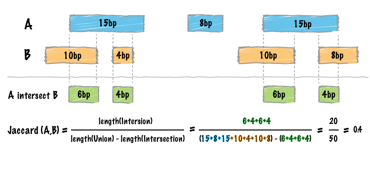
Calculate Jaccard statistics between the two BED data tables:

Image by bedtools

jaccard_bed(tbl_x, tbl_y)
#>    intersection union   jaccard n_intersections
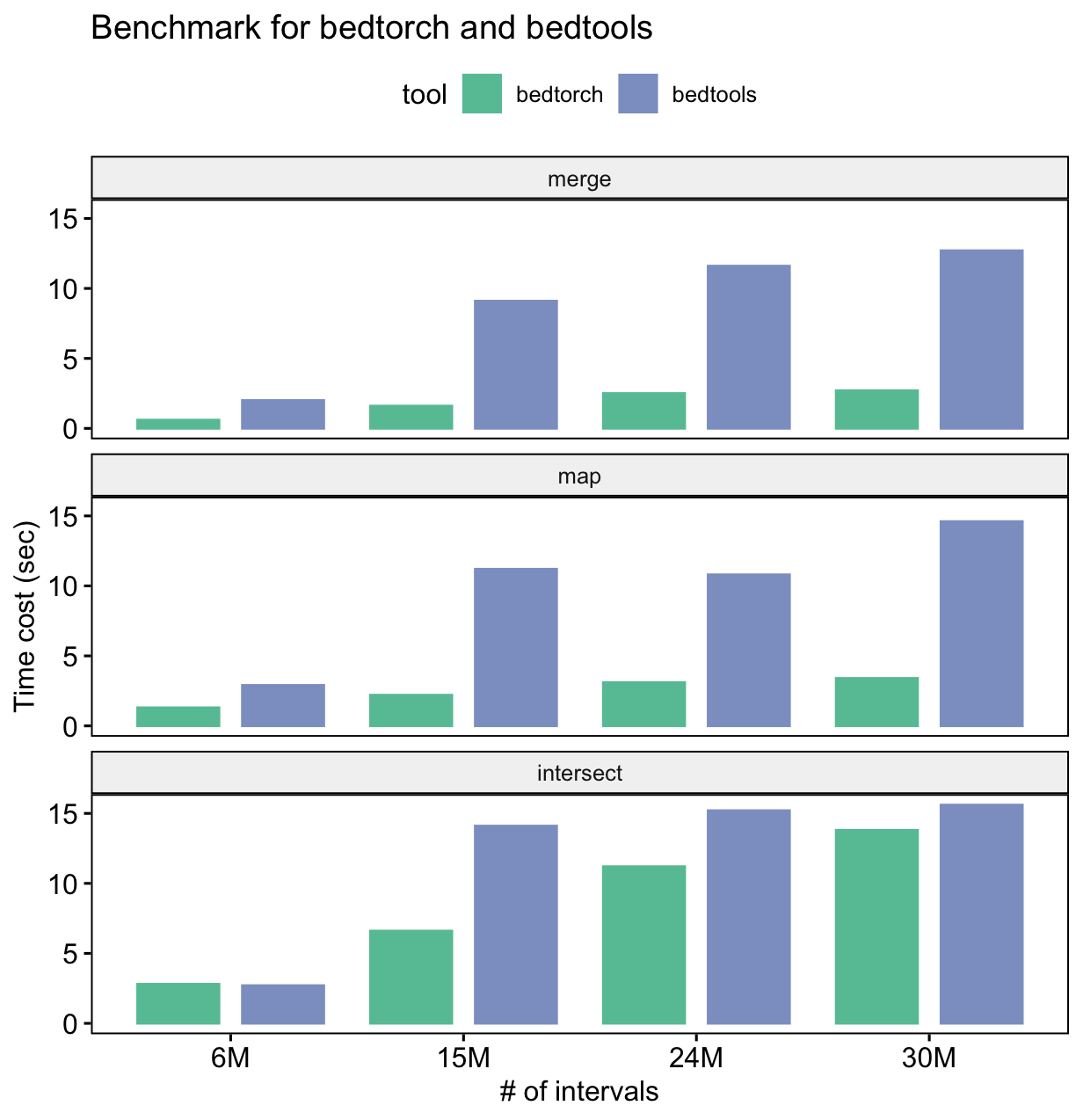
#> 1:           33    94 0.3510638               8

Performance

The following is the result of a simple benchmark for three common BED manipulations: merge, intersect and map.

Benchmark platform information:

• OS: macOS Big Sur 11.1
• CPU: 2.7 GHz Quad-Core Intel Core i7
• Memory: 16 GB LPDDR3

From the benchmark result, we can see that for all three tasks, bedtorch uses much less time than bedtools.

Note: this does not mean bedtools is indeed slower than bedtorch at performing the actual computation. Don’t forget bedtools requires large amount of disk IO, while bedtorch does not.

See also

Many features are inspired by bedtools. Thus, it’s helpful to get familiar with bedtool’s documentation: https://bedtools.readthedocs.io/en/latest/index.html