-
Notifications
You must be signed in to change notification settings - Fork 49
Choice of number of hybridizations
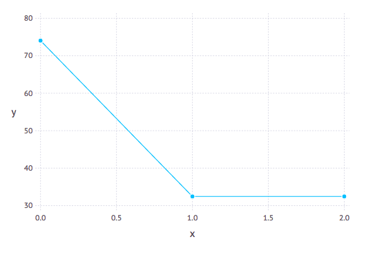
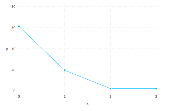
Model selection tools are necessary to estimate the number of hybridizations (h). We use the log pseudolikelihood profile with h. A sharp improvement is expected until h reaches the best value and a slower, linear improvement thereafter.
Unfortunately, there is no clear-cut criterion to determine what constitutes a large and 'significant' improvement in the pseudolikelihood score. Even with a regular likelihood, AIC and BIC are not quite appropriate, because they are not meant to accommodate the exploding number of models when h gets bigger (the network space grows very fast). That being said, the pattern of score improvement can be used heuristically.
The negative log pseudolikelihood score is an attribute of the network object:
net.loglik. The lower the better.
scores = [net0.loglik, net1.loglik, net2.loglik]
using RCall
R"pdf"("score-vs-h.pdf", width=4, height=4);
R"plot"(x=0:2, y=scores, type="b", xlab="number of hybridizations h",
        ylab="network score");
R"dev.off"();
Below are examples from 2 different data sets.


Recent work by Cai and Ane (2021) introduce a goodness-of-fit test for the adequacy of the multispecies network coalescent to see if a given population or species network explains the quartet concordance factor data adequately.
We need to install the new Julia package QuartetNetworkGoodnessFit.jl.
The commands below assume that we are in the directory for the
data set on 15 taxa: n15.gamma0.30.20.2_n300. So first, navigate to get there.
After the PhyloNetwork analyses on the other data set, we would need to do this:
cd ../n15.gamma0.30.20.2_n300/
We first read the CF table and get rid of the credibility intervals of the CFs:
using QuartetNetworkGoodnessFit, CSV
df = DataFrame(CSV.File("bucky-output/1_seqgen.CFs.csv"))
dat = df[:,[1,2,3,4,5,8,11,14]]
Then, we read the estimated network with 1 hybridization (our candidate network):
snaqnet1 = readTopology("snaq/net1_bucky.out")
rootatnode!(snaqnet1,"15")
We can plot the network:
using PhyloPlots
plot(snaqnet1,:R)
And now we fit the goodness-of-fit test (this could take a couple of minutes):
out = quarnetGoFtest!(snaqnet1, dat, false)The first component of the output out[1] corresponds to the p-value of the
overall goodness-of-fit test:
julia> out[1]
6.760380685802971e-6
This p-value implies that the candidate network (snaqnet1) does not explain the quartet
CFs adequately. This is not surprising as the data in n15.gamma0.30.20.2_n300
corresponds to simulated data from a network with 3 hybridizations, and snaqnet1 has only 1.
The other components in the output out (as well as input arguments) are explained in the documentation here.
Next: perform and summarize a bootstrap analysis
PhyloNetworks Workshop
- home
- example data
-
TICR pipeline:
from sequences to quartet CFs
- the data
- MrBayes on all genes
- BUCKy
- Quartet MaxCut
- RAxML & ASTRAL
- PhyloNetworks: from quartet CFs or gene trees to phylogenetic networks
- TICR test: is a population tree with ILS sufficient (vs network)?
- Continuous trait evolution on a network