-
Notifications
You must be signed in to change notification settings - Fork 49
TICR test: tree versus network?
Install R and the R package phylolm if you don't already have it. We need version 2.4 or higher. See its manual. Do this within R:
install.packages("phylolm")
or (preferred: to get the latest version on CRAN)
devtools::install_github("lamho86/phylolm") # if you already have devtools installed
Next, load phylolm (repeat at each new session):
library(phylolm)
The commands below assume that we are in the directory for the
data set on 15 taxa: n15.gamma0.30.20.2_n300. So first, navigate to get there.
After the PhyloNetwork analyses on the other data set, we would need to do this:
cd ../n15.gamma0.30.20.2_n300/
then start R from that directory. Alternatively, start R from anywhere and navigate to that directory within R.
The goal is to measure the goodness-of-fit of the coalescent model along a tree: does a tree model with ILS explains the gene tree discordance adequately? We will use gene tree discordance summarized on sets of 4 taxa: by the frequency (concordance factors) of the 3 quartets in gene trees.
In the previous sections we fitted a tree or a network to these quartet CFs. We can extract and
visualize the fit of the best tree (net0), or the fit of the best network with 1 reticulation
(net1) like this.
In julia:
buckyCF = readTableCF("bucky-output/1_seqgen.CFs.csv") # read observed quartet CF
net0b = readTopology("snaq/net0_bucky.out") # tree estimated earlier with snaq!
net1b = readTopology("snaq/net1_bucky.out") # network estimated earlier
topologyQPseudolik!(net0b, buckyCF)         # update the fitted CFs under net0
fitCF0 = fittedQuartetCF(buckyCF, :long)    # extract them to a data frame
topologyQPseudolik!(net1b, buckyCF)         # update the fitted CFs under net1
fitCF1 = fittedQuartetCF(buckyCF, :long)    # extract them to a data frame
The quartet CFs expected under a tree with ILS look like this:
julia> fitCF0
4095×7 DataFrames.DataFrame
│ Row  │ tx1 │ tx2 │ tx3 │ tx4 │ quartet │ obsCF      │ expCF      │
├──────┼─────┼─────┼─────┼─────┼─────────┼────────────┼────────────┤
│ 1    │ 10  │ 12  │ 7   │ 9   │ 12_34   │ 0.360093   │ 0.242426   │
│ 2    │ 10  │ 12  │ 7   │ 9   │ 13_24   │ 0.0648067  │ 0.242426   │
│ 3    │ 10  │ 12  │ 7   │ 9   │ 14_23   │ 0.5751     │ 0.515149   │
│ 4    │ 10  │ 12  │ 9   │ 15  │ 12_34   │ 0.236717   │ 0.127224   │
│ 5    │ 10  │ 12  │ 9   │ 15  │ 13_24   │ 0.70954    │ 0.745553   │
│ 6    │ 10  │ 12  │ 9   │ 15  │ 14_23   │ 0.0537467  │ 0.127224   │
⋮
│ 4089 │ 2   │ 1   │ 6   │ 14  │ 14_23   │ 0.02261    │ 0.04359    │
│ 4090 │ 13  │ 9   │ 1   │ 6   │ 12_34   │ 0.999943   │ 0.99699    │
│ 4091 │ 13  │ 9   │ 1   │ 6   │ 13_24   │ 3.66667e-5 │ 0.00150511 │
│ 4092 │ 13  │ 9   │ 1   │ 6   │ 14_23   │ 2.0e-5     │ 0.00150511 │
│ 4093 │ 13  │ 1   │ 15  │ 14  │ 12_34   │ 0.0176667  │ 0.0387301  │
│ 4094 │ 13  │ 1   │ 15  │ 14  │ 13_24   │ 0.01171    │ 0.0387301  │
│ 4095 │ 13  │ 1   │ 15  │ 14  │ 14_23   │ 0.970627   │ 0.92254    │
We can combine fitCF0 and fitCF1 into a single table, to contain the CFs observed in gene trees,
the CFs expected under a species tree, and the CFs expected under a network with 1 reticulation:
using DataFrames
fitCF = rename(fitCF0, :expCF => :expCF_net0); # rename column "expCF" to "expCF_net0"
fitCF[!,:expCF_net1] = fitCF1[!,:expCF];         # add new column "expCF_net1"
using CSV
CSV.write("snaq/fittedCF.csv", fitCF)        # export to .csv file
it looks like this:
julia> fitCF
4095×8 DataFrames.DataFrame
│ Row  │ tx1 │ tx2 │ tx3 │ tx4 │ quartet │ obsCF      │ expCF_net0 │ expCF_net1 │
├──────┼─────┼─────┼─────┼─────┼─────────┼────────────┼────────────┼────────────┤
│ 1    │ 10  │ 12  │ 7   │ 9   │ 12_34   │ 0.360093   │ 0.242426   │ 0.331138   │
│ 2    │ 10  │ 12  │ 7   │ 9   │ 13_24   │ 0.0648067  │ 0.242426   │ 0.0722191  │
│ 3    │ 10  │ 12  │ 7   │ 9   │ 14_23   │ 0.5751     │ 0.515149   │ 0.596643   │
│ 4    │ 10  │ 12  │ 9   │ 15  │ 12_34   │ 0.236717   │ 0.127224   │ 0.24523    │
│ 5    │ 10  │ 12  │ 9   │ 15  │ 13_24   │ 0.70954    │ 0.745553   │ 0.694199   │
│ 6    │ 10  │ 12  │ 9   │ 15  │ 14_23   │ 0.0537467  │ 0.127224   │ 0.0605708  │
⋮
│ 4089 │ 2   │ 1   │ 6   │ 14  │ 14_23   │ 0.02261    │ 0.04359    │ 0.0435896  │
│ 4090 │ 13  │ 9   │ 1   │ 6   │ 12_34   │ 0.999943   │ 0.99699    │ 0.996734   │
│ 4091 │ 13  │ 9   │ 1   │ 6   │ 13_24   │ 3.66667e-5 │ 0.00150511 │ 0.001633   │
│ 4092 │ 13  │ 9   │ 1   │ 6   │ 14_23   │ 2.0e-5     │ 0.00150511 │ 0.001633   │
│ 4093 │ 13  │ 1   │ 15  │ 14  │ 12_34   │ 0.0176667  │ 0.0387301  │ 0.0387295  │
│ 4094 │ 13  │ 1   │ 15  │ 14  │ 13_24   │ 0.01171    │ 0.0387301  │ 0.0387295  │
│ 4095 │ 13  │ 1   │ 15  │ 14  │ 14_23   │ 0.970627   │ 0.92254    │ 0.922541   │
We can read the table created in julia, "snaq/fittedCF.csv", and plot
it in different ways outside of Julia. We will stay in Julia though, and
arrange the fit to the 2 networks (h=0 and h=1) in a "long" format, and plot
it within Julia but via R and ggplot.
fitCF0[:, :h] = zeros(Int64, size(fitCF0, 1))
fitCF1[:, :h] = ones(Int64, size(fitCF1, 1))
fitCF = vcat(fitCF0, fitCF1)
fitCF
8190×8 DataFrames.DataFrame
│ Row │ tx1 │ tx2 │ tx3 │ tx4 │ quartet │ obsCF │ expCF │ h │
├──────┼─────┼─────┼─────┼─────┼─────────┼────────────┼───────────┼───┤
│ 1 │ 10 │ 12 │ 7 │ 9 │ 12_34 │ 0.360093 │ 0.242426 │ 0 │
│ 2 │ 10 │ 12 │ 7 │ 9 │ 13_24 │ 0.0648067 │ 0.242426 │ 0 │
│ 3 │ 10 │ 12 │ 7 │ 9 │ 14_23 │ 0.5751 │ 0.515149 │ 0 │
│ 4 │ 10 │ 12 │ 9 │ 15 │ 12_34 │ 0.236717 │ 0.127224 │ 0 │
⋮
│ 8187 │ 13 │ 9 │ 1 │ 6 │ 14_23 │ 2.0e-5 │ 0.001633 │ 1 │
│ 8188 │ 13 │ 1 │ 15 │ 14 │ 12_34 │ 0.0176667 │ 0.0387295 │ 1 │
│ 8189 │ 13 │ 1 │ 15 │ 14 │ 13_24 │ 0.01171 │ 0.0387295 │ 1 │
│ 8190 │ 13 │ 1 │ 15 │ 14 │ 14_23 │ 0.970627 │ 0.922541 │ 1 │
using RCall
@rlibrary ggplot2
ggplot(fitCF, aes(x=:obsCF, y=:expCF)) + geom_point(alpha=0.1) +
  xlab("CF observed in gene trees") + ylab("CF expected under tree (h=0) or network (h=1)") +
  facet_grid(R"~h", labeller = label_both)
# ggsave("fittedCFs.png", height=4, width=7)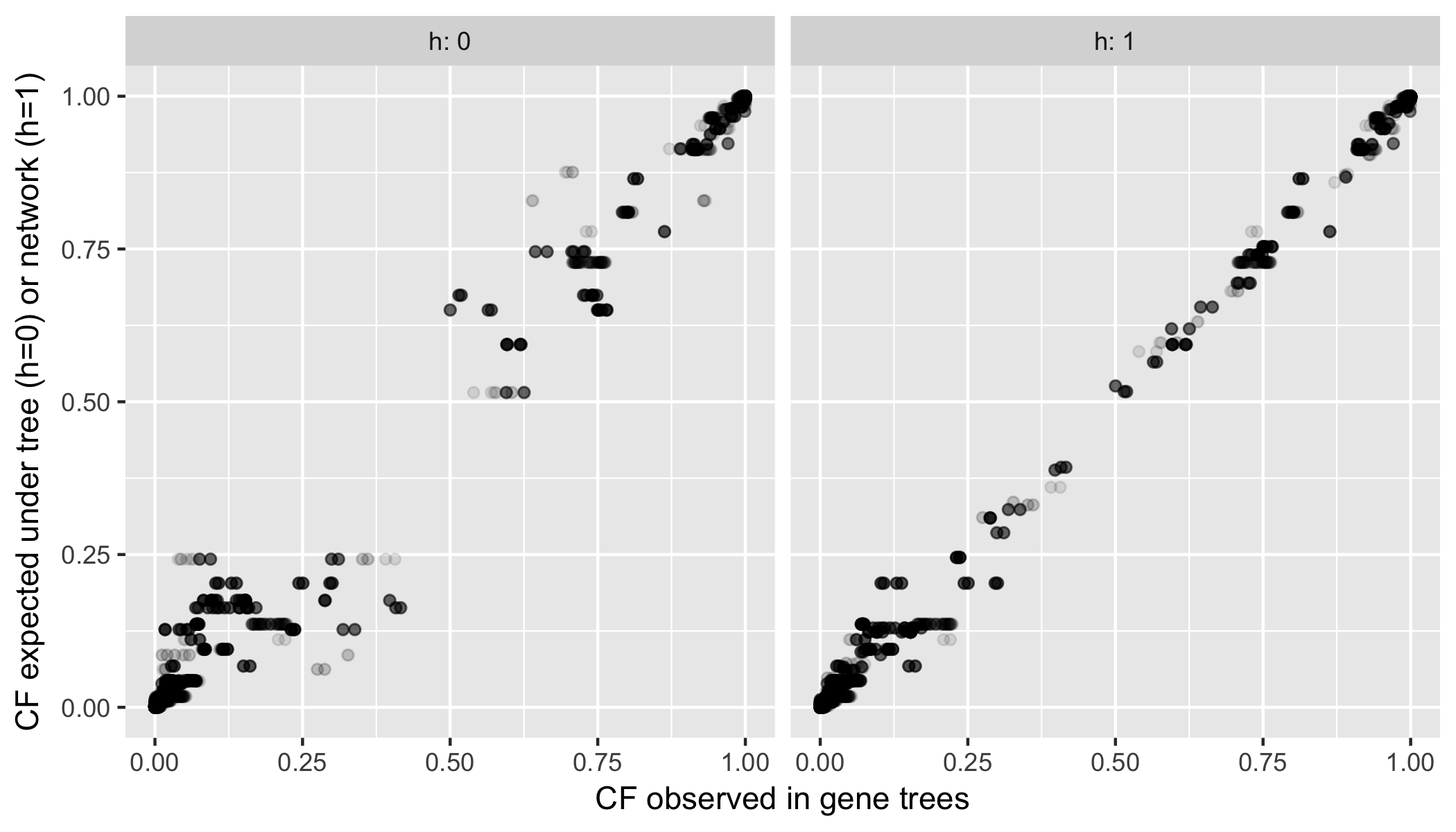
We see a clear improvement when a network is used, instead of a tree. The observed gene tree discordance (quartet CFs) is better explained using a network: points are closer to the diagonal. Is this improvement significant? The main statistical issue is the dependence between all these points.
- the 3 quartets from the same set of 4 taxa must have CFs that sum up to 1.
- different sets of 4 taxa do not provide independent quartet CFs.
The second point is not a problem for estimation. Only for significance testing.
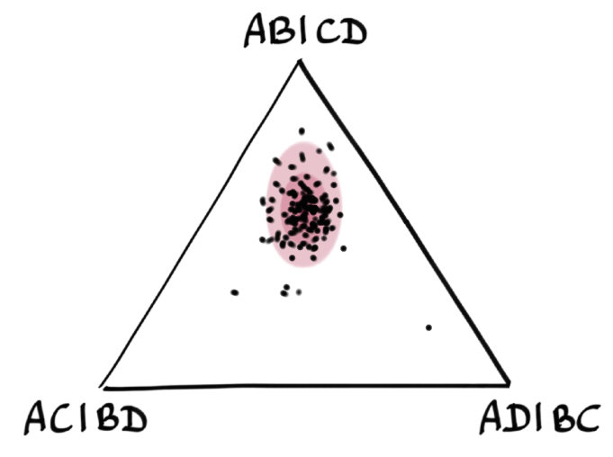
We solve the first issue by considering all 3 quartets from a given same 4-taxon set
simultaneously, and we assume a Dirichlet distribution for them, centered
at the values expected from the species tree and its coalescent units:


The "width" of the distribution is controlled by an unknown parameter α, to be estimated from the data. Large α: concentrated distribution. Discrepancy between observed CFs and values expected from the tree could be caused by
- gene tree estimation error (some due to incorrect molecular evolution model, long branch attraction for some 4-taxon sets, etc.)
- paralogy for some genes
- recombination within genes, etc.
Any of these would cause α to be lower: observed CFs further away from the expected CFs.
We estimate α using pseudo-maximum likelihood, combining all 4-taxon sets.
1 point = 1 four-taxon set = 3 quartet CFs below.
Then we calculate a p-value for each 4-taxon set, to measure how much of an outlier it might. With 15 taxa, we have 1365 4-taxon sets. So we expect 13 or 14 (1%) to look like outliers with an outlier p-values below 0.01. Just by chance. If we see many more than 13 or 14, it would mean that the tree does not fit the data.
The test needs more taxa to gain power. 5 taxa is definitely too low for instance, with only 5 four-taxon sets. That is too few to learn the distribution of quartet CFs and to detect outliers quartets. With 6 taxa, 15 4-taxon sets is also quite low.
Let's read the data in R: the quartet concordance factors estimated from the sequences.
> quartetCF = read.csv("bucky-output/1_seqgen.CFs.csv")
> dim(quartetCF)
[1] 1365   14     # there are 1365 4-taxon sets: 15 taxa, choose 4.
> head(quartetCF) # 'head' shows the first 6 rows only.
  taxon1 taxon2 taxon3 taxon4     CF12.34  CF12.34_lo CF12.34_hi    CF13.24 CF13.24_lo CF13.24_hi     CF14.23  CF14.23_lo CF14.23_hi ngenes
1     10     12      7      9 0.360093333 0.336666667 0.38333333 0.06480667 0.05000000  0.0800000 0.575100000 0.550000000 0.60000000    300
2     10     12      9     15 0.236716667 0.220000000 0.25333333 0.70954000 0.69333333  0.7266667 0.053746667 0.046666667 0.06333333    300
3     10     12     13     15 0.008003333 0.006666667 0.01333333 0.01677333 0.01666667  0.0200000 0.975226667 0.970000000 0.97666667    300
4     10     12     11     13 0.019756667 0.016666667 0.02333333 0.97271667 0.96666667  0.9766667 0.007526667 0.006666667 0.01000000    300
5     10     12      5     13 0.008003333 0.006666667 0.01333333 0.97522667 0.97000000  0.9766667 0.016773333 0.016666667 0.02000000    300
6     10     12      8     15 0.231126667 0.216666667 0.24666667 0.72830333 0.71333333  0.7433333 0.040570000 0.033333333 0.05000000    300
We need to get rid of credibility intervals of CFs, to get the estimates of CFs in columns 5-7. We also need to make sure that taxon names are interpreted as names rather than numbers:
> dat = quartetCF[, c(1:4, 5, 8, 11)]
> for (i in 1:4){ dat[,i] = factor(dat[,i])}
> head(dat)
  taxon1 taxon2 taxon3 taxon4     CF12.34    CF13.24     CF14.23
1     10     12      7      9 0.360093333 0.06480667 0.575100000
2     10     12      9     15 0.236716667 0.70954000 0.053746667
3     10     12     13     15 0.008003333 0.01677333 0.975226667
4     10     12     11     13 0.019756667 0.97271667 0.007526667
5     10     12      5     13 0.008003333 0.97522667 0.016773333
6 10 12 8 15 0.231126667 0.72830333 0.040570000We also read in the species tree to be tested. This tree needs to have branch lengths in coalescent units (number of generations divided by effective population size). For example, we might use
- the species tree estimated by ASTRAL, which has branch lengths in coalescent units (using ASTRAL v4.10.0 or higher)
- or the species tree estimated by PhyloNetworks with h=0 hybridizations.
To get the astral tree, we read in all trees in the astral results file and only keep the last tree: number 102. That's because ASTRAL outputs the 100 bootstrap trees first, then their consensus, and finally the tree from the original data annotated with node support and branch lengths.
> library(phylolm)
> astraltree = read.tree("astral/astral.tre")[[102]]
> astraltree

Phylogenetic tree with 15 tips and 14 internal nodes.

Tip labels:
	14, 1, 15, 3, 2, 6, ...
Node labels:
	, NA, 100.0, 100.0, 100.0, 100.0, ...

Rooted; includes branch lengths.

> plot(astraltree)
Error in .nodeDepthEdgelength(Ntip, Nnode, z$edge, Nedge, z$edge.length) :
  NA/NaN/Inf in foreign function call (arg 6)
> plot(astraltree, use.edge.length=F) # no problem!
> edgelabels(round(astraltree$edge.length,3))
The first plotting error was because some branch lengths are there, and others are not! External branch lengths cannot be estimated (in coalescent units) unless we have multiple individuals per species. In the plot we notice that the arbitrary outgroup used by ASTRAL was wrong, so we re-root the tree, with the correct outgroup "15":
astraltree = root(astraltree, "15")
plot(astraltree, use.edge.length=F)
edgelabels(round(astraltree$edge.length,3), frame="none", adj=c(0.5,0))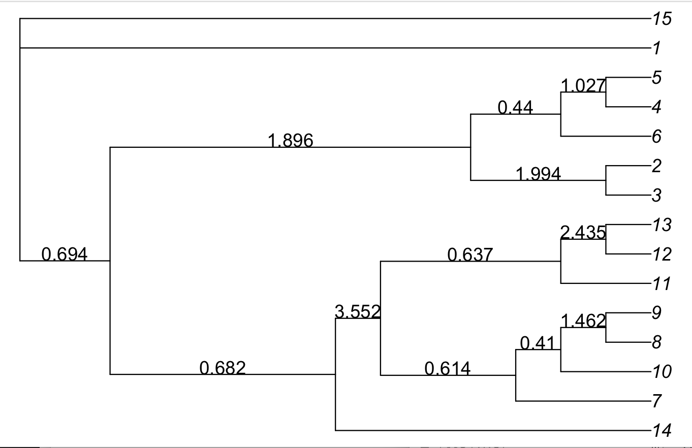
We can repeat the same procedure to read in the species tree from PhyloNetworks, but this time we keep the very first tree read from the output file:
##snaqtree = read.tree("snaq/net0_bucky.out")[[1]] ## we get error now, ignore for now!
##snaqtree = root(snaqtree, "15")
##plot(snaqtree, use.edge.length=F)
##edgelabels(round(snaqtree$edge.length,3), frame="none", adj=c(0.5,0))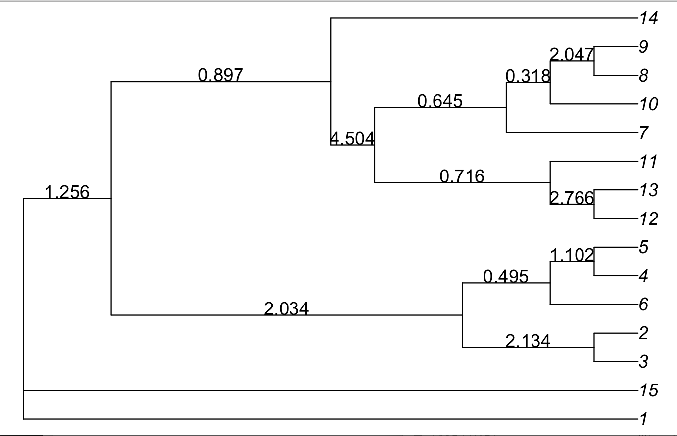
Both trees have the same topology. They differ a bit in branch lengths. Below we use the astral tree only, but feel tree to repeat with the snaq tree to see if results are robust to estimation error in branch lengths.
This is to learn which edges are along the internal path of which quartets. It speeds up all future calculations.
> astralprelim = test.tree.preparation(dat, astraltree)
determining tree traversal node post-order... done.
calculating matrix of descendant relationships... done.
calculating matrix of edges spanned by each quartet... done.
> Ntaxa = length(astraltree$tip.label) # 15 of course
> astral.internal.edges = which(astraltree$edge[,2] > Ntaxa)
> astral.internal.edges # indices of internal edges: those that need a length
[1] 1 2 4 5 7 9 12 14 17 18 21 23 # in coalescent unitsThis is a goodness-of-fit test, assuming that the given branch lengths (in coalescent units) are correct.
> res <- test.one.species.tree(dat,astraltree,astralprelim,edge.keep=astral.internal.edges)
The chi-square test is significant at level .05,
but there is a deficit of outlier quartets (with outlier p-value<=0.01).
This pattern does not have a simple evolutionary explanation.
> res[1:6]
$alpha
[1] 59.06629

$minus.pll
[1] -7280.939

$X2
[1] 28.03297

$chisq.pval
[1] 3.574625e-06

$chisq.conclusion
[1] "The chi-square test is significant at level .05,\nbut there is a deficit of outlier quartets (with outlier p-value<=0.01).\nThis pattern does not have a simple evolutionary explanation.\n"

$outlier.table
           .01  .05   .10  large
observed 13.00 92.0 57.00 1203.0
expected 13.65 54.6 68.25 1228.5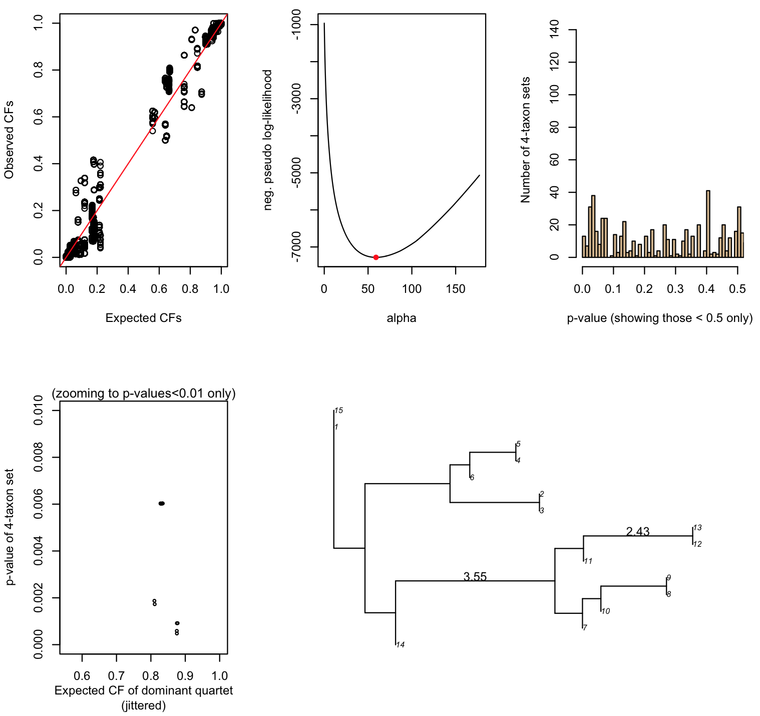
Despite the output message, the number of outlier p-values below 0.01 is just as expected, and there is an excess of outlier p-values between 0.01-0.05.
Looking at the outlier 4-taxon sets can point us to taxa that do not fit the tree model with ILS.
> outlier.4taxa.01 <- which(res$outlier.pvalues < 0.01)
> length(outlier.4taxa.01)
[1] 13 # 13 4-taxon sets have an outlier p-value below 0.01
> q01 = as.matrix(quartetCF[outlier.4taxa.01,1:4])
> q01
     taxon1 taxon2 taxon3 taxon4
40       10     12     11      8
60       10     11      7     13
63       10     11      8     13
64       10     12     11      7
92       10     12     11      9
131      10     11     13      9
370      10      1     15     14
701      12      1     15     14
865      11      1     15     14
1105      7      1     15     14
1152      8      1     15     14
1350      9      1     15     14
1365     13      1     15     14
> sort(table(as.vector(q01)),decreasing=TRUE)

 1 10 11 14 15 12 13  7  8  9  # this is the taxon name
 7  7  7  7  7  4  4  3  3  3  # number of outlier 4-taxon sets in which the taxon appears
All the outlier quartets with p-value <0.01 involve taxa 1,14,15 and another taxon; or taxa 10, 11, 12 or 13, and one of {7,8,9}.
In fact, the true network used to generate the data has ancient gene flow near the divergences between taxa 1, 14 and 15. Also, taxon 10 is sister to {8,9} but received gene flow from taxon 11, which is sister to {12,13}. To get more info, we can compare the observed concordance factors (estimated from the data) to those expected from ILS on the tree:
> cbind(
+    dat[outlier.4taxa.01,],       # taxon names and observed CFs
+    res$cf.exp[outlier.4taxa.01,] # CFs expected from the tree
+ )
     taxon1 taxon2 taxon3 taxon4    CF12.34    CF13.24   CF14.23   expCF12.34 expCF13.24 expCF14.23
40       10     12     11      8 0.01749333 0.27515333 0.7073533   0.06327315 0.06327315 0.87345369
60       10     11      7     13 0.32781000 0.63859000 0.0336000   0.09536698 0.80926604 0.09536698
63       10     11      8     13 0.27512000 0.70733000 0.0175500   0.06327315 0.87345369 0.06327315
64       10     12     11      7 0.03345000 0.32629333 0.6402533   0.09536698 0.09536698 0.80926604
92       10     12     11      9 0.01343333 0.28756000 0.6990033   0.06327315 0.06327315 0.87345369
131      10     11     13      9 0.28737000 0.01748667 0.6951433   0.06327315 0.06327315 0.87345369
370      10      1     15     14 0.01766333 0.01172667 0.9706100   0.08415475 0.08415475 0.83169050
701      12      1     15     14 0.01766667 0.01171000 0.9706267   0.08415475 0.08415475 0.83169050
865      11      1     15     14 0.01766333 0.01172667 0.9706100   0.08415475 0.08415475 0.83169050
1105      7      1     15     14 0.01768667 0.01169667 0.9706167   0.08415475 0.08415475 0.83169050
1152      8      1     15     14 0.01763000 0.01171667 0.9706533   0.08415475 0.08415475 0.83169050
1350      9      1     15     14 0.01763000 0.01171667 0.9706533   0.08415475 0.08415475 0.83169050
1365     13      1     15     14 0.01766667 0.01171000 0.9706267   0.08415475 0.08415475 0.83169050
For all outliers involving taxa 10 and 11 (first 7 rows), 10 and 11 are sister to each other in a greater proportion of genes (obs CFs) than expected from the tree.
> outlier.4taxa.05 <- which(res$outlier.pvalues < 0.05)
> length(outlier.4taxa.05)
[1] 105
> q05 = as.matrix(quartetCF[outlier.4taxa.05,1:4])
> head(q05)
   taxon1 taxon2 taxon3 taxon4
11     10     12     11     15
20     10     11      7      6
33     10     12     11     14
40     10     12     11      8
46     10     12     11      5
53     10     11      7      1
> sort(table(as.vector(q05)),decreasing=TRUE)
 1 15 11 10  7 12 13  8  9 14  2  3  4  5  6
53 53 48 44 36 27 27 26 18 18 14 14 14 14 14
> sum(apply(q05,1,function(x){"1" %in% x  & "15" %in% x}))
[1] 47
> sum(apply(q05,1,function(x){"10" %in% x & "11" %in% x}))
[1] 38

> clade10.13 = c("10", "11", "12", "13")
> table(apply(q05,1,function(x){length(intersect(x, clade10.13))}))

 0  1  2  3 # number of taxa in the clade "10","11","12","13"
23 40 20 22 # number of outlier 4-taxon sets
> 40+20+22
[1] 82      # 82 outliers have 1,2 or 3 of their 4 taxa in the clade

> clade7.9 = c("7", "8", "9")
> table(apply(q05,1,function(x){length(intersect(x, clade7.9))}))

 0  1  2  # number of taxa in the clade "7","8","9"
45 40 20  # 40 outliers have exactly one of 7,8 or 9, and 20 outliers have exactly 2 of them.
When we expand the list of outlier 4-taxon sets to those with p-value below 0.05, the list is much longer, but the same 2 patterns appear. About half of outliers (47 out 105) involve both taxa 1 and 15, 44 involve the hybrid taxon 10, and 38 involve both taxa 10 and 11. The vast majority of these outlier 4-taxon sets (82 out of 105) involve at least one taxon from the group 10-14.
Note that we can now run the TICR test on julia with the
QuartetNetworkGoodnessFit.jl package.
using QuartetNetworkGoodnessFit, CSV, PhyloPlots
df = DataFrame(CSV.File("bucky-output/1_seqgen.CFs.csv"))
dat = df[:,[1,2,3,4,5,8,11]]
astraltree = readMultiTopology("astral/astral.tre")[102] # main tree with BS as node labels
rootatnode!(astraltree,"15")
plot(astraltree,:R, showEdgeLength=true)
out = ticr!(astraltree,dat,false)
The first entry of the out object has the p-value of the overall goodness-of-fit test:
julia> out[1]
2.5095827563325576e-6
This p-value shows that the candidate tree (astraltree) is not a good fit to the quartet CFs.
This is not surprising since the data in n15.gamma0.30.20.2_n300
corresponds to simulated data from a network with 3 hybridizations, and astraltree has 0 hybridizations.
An explanation of all the output components (as well as input arguments) can be found in the documentation here.
PhyloNetworks Workshop
- home
- example data
-
TICR pipeline:
from sequences to quartet CFs
- the data
- MrBayes on all genes
- BUCKy
- Quartet MaxCut
- RAxML & ASTRAL
- PhyloNetworks: from quartet CFs or gene trees to phylogenetic networks
- TICR test: is a population tree with ILS sufficient (vs network)?
- Continuous trait evolution on a network