SNaQ

Types of input

To run SNaQ, you need

• data extracted from sequence alignments:

  • a list of estimated unrooted gene trees (e.g. from RAxML), or
  • a table of concordance factors (CF) (e.g. from BUCKy)

• a starting topology (e.g. from Quartet MaxCut or ASTRAL, or RAxML tree from a single gene...)

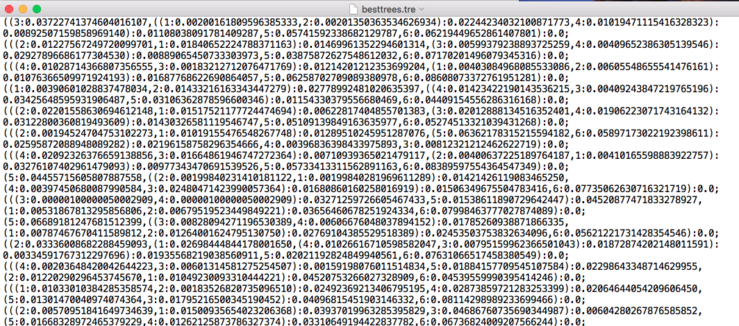
List of estimated unrooted gene trees: plain text file with one tree per line in parenthetical format.

Table of CF: plain text file or comma-separated file, obtained from TICR pipeline.

Starting topology: tree or network in parenthetical format

Network estimation

SNaQ estimates unrooted explicit networks with a maximum pseudolikelihood approach.

Remember you need to load the packages if you are just starting Julia:

using PhyloNetworks
using PhyloPlots

Read the data into Julia:

buckyCF = readTableCF("bucky-output/1_seqgen.CFs.csv")

or

raxmlCF = readTrees2CF("raxml/besttrees.tre", writeTab=false, writeSummary=false)

For large files, we can use the alternative (more efficient) code:

trees = readMultiTopology("raxml/besttrees.tre")
q,t = countquartetsintrees(trees)
df = writeTableCF(q,t)
raxmlCF = readTableCF(df)

For the starting topology, the Quartet MaxCut tree is saved in one file, whereas the ASTRAL tree is saved at the end of a list of bootstrap trees:

tre = readTopology("bucky-output/1_seqgen.QMC.tre")

or

astraltree = readMultiTopology("astral/astral.tre")[102] # main tree with BS as node labels

Estimate the best network from bucky's quartet CF and hmax number of hybridizations (make sure to have a folder called snaq in the working directory):

net0 = snaq!(tre,  buckyCF, hmax=0, filename="snaq/net0_bucky", seed=123)
net1 = snaq!(net0, buckyCF, hmax=1, filename="snaq/net1_bucky", seed=456)

We want to continue with hmax=2, but faster. Let's tell Julia to use multiple threads to parallelize individual runs. We can check the number of threads available on our machine by using the command sysctl -n hw.ncpu on the OSX terminal, while either nproc or lscpu should work on the Linux terminal; we will assume our machine has only two threads available. When we do so, snaq! will send its different runs to different processors. The screen output is a little different.

using Distributed
addprocs(2) # tells Julia to add 2 threads
@everywhere using PhyloNetworks # tells these threads to load the PhyloNetworks package for themselves
net2 = snaq!(net1, buckyCF, hmax=2, filename="snaq/net2_bucky", seed=789, runs=5) # different runs will be sent to different cores

By default, each optimization will do 10 runs (runs=10), but we choose runs=5 for speed in the tutorial.

To estimate the best network from raxml's gene trees, the command is the same, except for the input data (and perhaps for the output file where we want the results to do):

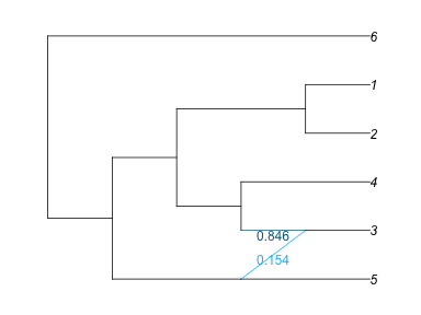
net1r = snaq!(net0, raxmlCF, hmax=1, filename="snaq/net1_raxml")

We can plot the estimated networks:

using PhyloPlots
plot(net0, :R);

again, if a plot window didn't pop up, an alternative is to save the plot as a pdf and open it outside of julia:

R"pdf"("plot3-net0.pdf", width=3, height=3);
plot(net0, :R);
R"dev.off()";

But taxon 6 was the outgroup, and it does not show as an outgroup. This is okay, because SNaQ infers an unrooted (or rather, semi-rooted) network. Let's reroot all of our networks with our outgroup.

# R"pdf"("plot4-net012.pdf", width=8, height=3); # to save as pdf if needed
R"layout(matrix(1:3,1,3))"; # to have a panel of 3 plots in 1 figure
R"par"(mar=[0.1,0.1,0.1,0.5]);
rootatnode!(net0, "6")
plot(net0, :R);
rootatnode!(net1, "6")
plot(net1, :R);
rootatnode!(net2, "6")
plot(net2, :R);
# R"dev.off()";

The minor hybrid edge crosses other edges, so let's rotate the top/down sisters to make the plot nicer. First, we need to know the number of the node around which we want to rotate edges.

# R"pdf"("plot5-net1.pdf", width=8, height=3); # to save as pdf if needed
R"layout"([1 2 3]);  # for 3 plots in 1 figure. [1 2 3] is a 1x3 matrix (of plots here)
R"par"(mar=[0.1,0.1,0.1,0.5]);
plot(net1, :R, showNodeNumber=true);
rotate!(net1, -3)
plot(net1, :R);
plot(net1, :R, showGamma=true);
# R"dev.off()";

Output files

• .out file: contains the best network among all runs, and the best network per run, includes also the pseudolikelihood score and the computation time.

  (1,2,((4,(3)#H7:::0.8455008017543593):10.0,(6,(5,#H7:::0.15449919824564068):1.3478059001640503):0.8097232227650086):8.859048876499543); -Ploglik = 32.44166815275073
  Dendroscope: (1,2,((4,(3)#H7):10.0,(6,(5,#H7):1.3478059001640503):0.8097232227650086):8.859048876499543);
  Elapsed time: 279.945323758 seconds, 10 attempted runs
  -------
  List of estimated networks for all runs (sorted by log-pseudolik; the smaller, the better):
  (1,2,((4,(3)#H7:::0.8455008017543593):10.0,(6,(5,#H7:::0.15449919824564068):1.3478059001640503):0.8097232227650086):8.859048876499543);, with -loglik 32.44166815275073
  (1,2,((6,(5,#H7:::0.15449929246440022):1.3478048315566553):0.8097228561399494,(4,(3)#H7:::0.8455007075355998):10.0):8.858993407546471);, with -loglik 32.44166815276231
  (1,2,((6,(5,#H7:::0.15449950311468977):1.347797935277818):0.8097218999238613,(4,(3)#H7:::0.8455004968853103):10.0):8.859068579213334);, with -loglik 32.44166815299586
  (1,2,((4,(3)#H7:::0.8455028784370155):10.0,(6,(5,#H7:::0.15449712156298445):1.3478623437305024):0.8097829889895752):9.686329026439614);, with -loglik 32.44681878021907
  (1,2,((4,(3,#H7:0.0::0.12596024349126436):10.0):6.998525545802376,((5,6):0.6706815043923903)#H7:0.02644187240118026::0.8740397565087357):8.802233330267686);, with -loglik 38.47631220369748
  (1,2,((4,(3,#H7:0.0::0.12669655104300853):5.137606913234892):9.662626208222877,((5,6):0.6721814535915894)#H7:0.025109110453433996::0.8733034489569915):9.999190138600072);, with -loglik 38.48682416318879
  (1,2,(((5,6):0.48745060060410667,(3,(4)#H7:::0.8562805766179749):7.459921008438409):5.783680919305781,#H7:::0.14371942338202517):9.999680749757447);, with -loglik 39.165297532921166
  (2,1,(((3,(4)#H7:::0.856702302080893):6.842325499857021,(5,6):0.48745123178986577):8.84844751722053,#H7:::0.1432976979191069):9.705601003398822);, with -loglik 39.165297532966704
  (2,1,(((3,(4)#H7:::0.856716182654851):6.827117792791621,(5,6):0.4874498177842928):9.980179092466777,#H7:::0.14328381734514894):8.210595868229708);, with -loglik 39.16529753331082
  (1,2,(((4,3):1.4572675240847626,(5,(6)#H7:::0.7580193251190865):1.31560016434676):9.979843400401359,#H7:::0.2419806748809134):7.098369544865319);, with -loglik 40.717647931470985
  -------
  

• .networks file: contains the networks obtained by switching the hybrid node inside each cycle (because of potential identifiabiliy issues).

  (1,2,((4,(3)#H7:::0.8455008017543593):10.0,(6,(5,#H7:::0.15449919824564068):1.3478059001640503):0.8097232227650086):8.859048876499543);, with -loglik 32.44166815275073 (best network found, remaining sorted by log-pseudolik; the smaller, the better)
  (1,2,((4,(3,#H7:::0.17493951971036137):1.0060603344148846):2.251254356415373,(6,(5)#H7:::0.8250604802896386):1.1591996918589282):8.12886551182064);, with -loglik 38.56527982546186
  (1,2,(#H7:::0.17739396674858887,(6,(5,(3,(4)#H7:::0.8226060332514111):8.054305321403243):0.033502492781334416):3.6927109132625615):5.3702784570971644);, with -loglik 86.3478945657121
  (#H7:9.374999128965698::0.42574056046963116,4,(3,(5,(6,((1,2):8.859258713532823)#H7:0.8096935556192413::0.5742594395303688):1.8395730576771743):3.5649233234248294):0.4815558034289685);, with -loglik 119.5463693848075
  (1,2,((4,(3,(5,(6)#H7:::0.5814752796026457):2.7705818610565034):0.0):1.7681838379153163,#H7:::0.41852472039735433):8.365569611574916);, with -loglik 226.60240574282727
  

  
  

• .log file: description of each run, convergence criterion, seed information
  

• .err file: seed information on runs that failed, empty when nothing failed.

  In the case of a failed run, for example: Total errors: 1 in seeds [4545], you could run the following function on the same settings that caused the error: snaqDebug(tree,data,seed=4545) (to help us debug).

Suggestions

• For big datasets, do only one run first to get an idea of computing time:

  net1 = snaq!(net0, buckyCF, hmax=1, filename="snaq/net1_bucky", runs=1)

• Increase the number of hybridizations sequentially: hmax=0,1,2,..., and use the best network at h-1 as starting point to estimate the best network at h.
• Whenever possible, do many independent runs (default runs=10) to avoid getting stuck on local maxima. We do not need to do all runs sequentially. We can parallize by doing different runs on different cores (or computers). If we are on a machine or on a cluster that has many different cores, we can ask Julia to use these multiple cores, and snaq! will send different runs to different cores, like we did earlier.
• For long jobs, run as a script in the terminal: julia runSNaQ.jl, arguments to the script are passed to Julia as a vector called ARGS. See the example script runSNaQ.jl in the folder data_results/scripts/. more on this topic in the package doc.

Troubleshooting

The network does not make any sense!

Recall:

• The root is meaningless, use the rooting functions (more here)
• Identifiability issues: check out the .networks file, and its pseudolikelihood scores (more here).

  vnet = readMultiTopology("snaq/net1_bucky.networks")
  plot(vnet[1], :R) # best network
  rootatnode!(vnet[1],"6")
  rootatnode!(vnet[2],"6")
  # R"pdf"("plot6-boot.pdf", width=6, height=3); # to save as pdf if needed
  R"layout"([1 2]); # [1 2] is a 1x2 matrix. [1,2] is a vector of length 2
  R"par"(mar=[0.1,0.1,0.1,0.5]);
  plot(vnet[1], :R);
  plot(vnet[2], :R);
  #R"dev.off"();

  looking at the plots: the difference between the best and second-scoring networks is the direction of gene flow. To see the likelihood scores of these alternative networks:

  ; less snaq/net1_bucky.networks
  ; grep -Eo "with -loglik [0-9]+.[0-9]+" snaq/net1_bucky.networks

• Level-1 assumption: no intersecting cycles, so maybe no more hybridizations can be added if number of taxa is small
  
• The bigger the network to estimate, the more genes are needed (compare bootstrap results between 30 genes and 300 genes).

Documentation

• General documentation here
• Inside Julia: ?plot

Help/bugs/errors

• PhyloNetworks google group
• check the issues open on GitHub, open a new one if the problem that you are encountering is new
• email us

Next: how to choose the number of reticulations.