{% include list.liquid all=true %}
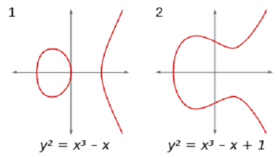
In number theory, the partition functionp(n) represents the number of possible partitions of a non-negative integer n. Integers can be considered either in themselves or as solutions to equations (Diophantine geometry).
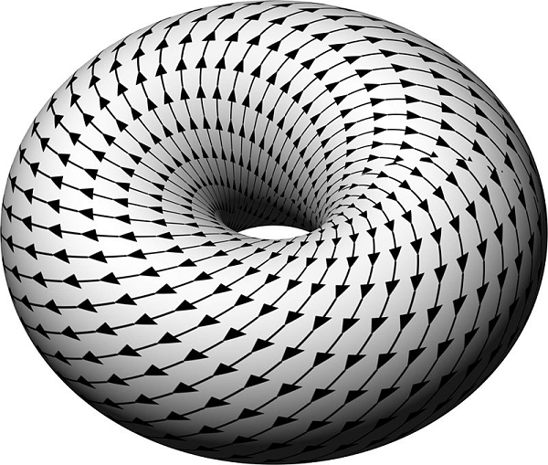
The central problem is to determine when a Diophantine equation has solutions, and if it does, how many. Two examples of an elliptic curve, that is, a curve of genus 1 having at least ***one rational point***. Either graph can be seen as a slice of a torus in four-dimensional space _([Wikipedia](https://en.wikipedia.org/wiki/Number_theory#Diophantine_geometry))_.
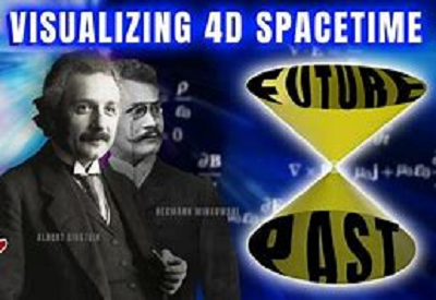
One of the main reason is that one does not yet have a mathematically complete example of a quantum gauge theory in four-dimensional space-time. It is even a sign that Einstein’s equations on the energy of empty space are somehow incomplete.
Throughout his life, Einstein published hundreds of books and articles. He published more than 300 scientific papers and 150 non-scientific ones. On 5 December 2014, universities and archives announced the release of Einstein's papers, comprising more than 30,000 unique documents _([Wikipedia](https://en.wikipedia.org/wiki/Albert_Einstein#Scientific_career))_.
Speculation is that the unfinished book of Ramanujan's partition, series of Dyson's solutions and hugh of Einstein's papers tend to solve it.
Dyson introduced the concept in the context of a study of certain congruence properties of the partition function discovered by the mathematician Srinivasa Ramanujan who the one that found the interesting behaviour of the taxicab number 1729.
The concept was introduced by [Freeman Dyson](https://en.wikipedia.org/wiki/Freeman_Dyson)in a paper published in the journal [Eureka](https://en.wikipedia.org/wiki/Eureka_(University_of_Cambridge_magazine)). It was [presented](https://en.wikipedia.org/wiki/Rank_of_a_partition#cite_note-Dyson-1) in the context of a study of certain [congruence](https://en.wikipedia.org/wiki/Congruence_relation) properties of the [partition function](https://en.wikipedia.org/wiki/Partition_function_(number_theory)) discovered by the Indian mathematical genius [Srinivasa Ramanujan](https://en.wikipedia.org/wiki/Srinivasa_Ramanujan). _([Wikipedia](https://e
n.wikipedia.org/wiki/Rank_of_a_partition))_
Young tableaux were introduced by Alfred Young, a mathematician at Cambridge University, in 1900. They were then applied to the study of the symmetric group. Their theory was further developed by many mathematicians, including W. V. D. Hodge
In _[number theory](https://gist.github.com/eq19/e9832026b5b78f694e4ad22c3eb6c3ef#number-theory)_ and combinatorics, [rank of a partition](https://en.wikipedia.org/wiki/Rank_of_a_partition) of a positive integer is a certain integer associated with the partition meanwhile the [crank of a partition](https://en.wikipedia.org/wiki/Crank_of_a_partition) of an integer is a certain integer associated with that partition _([Wikipedia](https://en.wikipedia.org/wiki/Freeman_Dyson#Crank_of_a_partition))_.

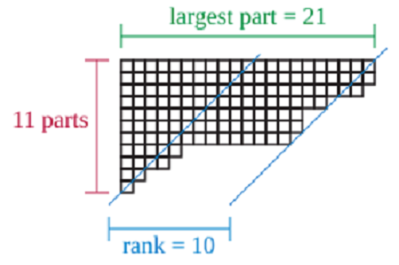
In mathematics, the rank of a partition is the number obtained by subtracting the number of parts in the partition from the largest part in the partition.
On the other hand, one does not yet have a mathematically complete example of a quantum gauge theory in 4D Space vs Time, nor even a precise definition of quantum gauge theory in four dimensions. Will this change in the 21st century? We hope so! _([Clay Institute's - Official problem description](https://claymath.org/sites/default/files/yangmills.pdf))_.

25 + 19 + 13 + 7 = 64 = 8 × 8 = 8²

The True Prime Pairs:
(5,7), (11,13), (17,19)

|--------------- 7¤ ---------------|
|-------------- {89} --------------|👈
+----+----+----+----+----+----+----+----+----+----+----+----+----+----+
|  5 |  7 | 11 |{13}| 17 | 19 | 17 |{12}| 11 | 19 |{18}| 18 | 12 |{13}|
+----+----+----+----+----+----+----+----+----+----+----+----+----+----+
        ∆         ∆      |---- {48} ----|---- {48} ----|---- {43} ----|👈
        7        13      |----- 3¤ -----|----- 3¤ -----|----- 3¤ -----|
                         |-------------------- 9¤ --------------------|
                            ∆                               |-- 25 ---|
                           19                                    ∆
                                                               5 x 5
SU(5) fermions of standard model in 5+10 representations. The sterile neutrino singlet's 1 representation is omitted. Neutral bosons are omitted, but would occupy diagonal entries in complex superpositions. X and Y bosons as shown are the opposite of the conventional definition


$True Prime Pairs:
(5,7), (11,13), (17,19)

     |    168    |    618    |
-----+-----+-----+-----+-----+                                             ---
 19¨ |  3¨ |  4¨ |  6¨ |  6¨ | 4¤  ----->  assigned to "id:30"             19¨
-----+-----+-----+-----+-----+                                             ---
 17¨ |  5¨ |  3¨ | ..  |  .. | 4¤ ✔️ --->  assigned to "id:31"              |
     +-----+-----+-----+-----+                                              |
{12¨}|  .. |  .. |  2¤ (M & F)     ----->  assigned to "id:32"              |
     +-----+-----+-----+                                                    |
 11¨ |  .. |  .. |  .. | 3¤ ---->  Np(33)  assigned to "id:33"  ----->  👉 77¨
-----+-----+-----+-----+-----+                                              |
 19¨ |  .. |  .. |  .. |  .. | 4¤  ----->  assigned to "id:34"              |
     +-----+-----+-----+-----+                                              |
{18¨}|  .. |  .. |  .. | 3¤        ----->  assigned to "id:35"              |
     +-----+-----+-----+-----+-----+-----+-----+-----+-----+               ---
 43¨ |  .. |  .. |  .. |  .. |  .. |  .. |  .. |  .. |  .. | 9¤ (C1 & C2)  43¨
-----+-----+-----+-----+-----+-----+-----+-----+-----+-----+               ---
139¨ |  1     2     3  |  4     5     6  |  7     8     9  |
                    Δ                 Δ                 Δ
Family Number Group +3, +6, +9 being activated by the Aetheron Flux Monopole Emanations, creating Negative Draft Counterspace, Motion and Nested Vortices.) _([RodinAerodynamics](https://rense.com/RodinAerodynamics.htm))_

This idea was taken as the earliest in 1960s Swinnerton-Dyer by using the University of Cambridge Computer Laboratory to get the number of points modulo p (denoted by Np) for a large number of primes p on elliptic curves whose rank was known.
From these numerical results ***the conjecture predicts that the data should form a line of slope equal to the rank of the curve***, which is 1 in this case drawn in red in red on the graph _([Wikipedia](https://en.wikipedia.org/wiki/Birch_and_Swinnerton-Dyer_conjecture#Current_status))_.
Dyson discovered that the eigenvalue of these matrices are spaced apart in exactly the same manner as _[Mo Unfortunately the rotation of this eigenvalues deals with four-dimensional space-time which was already a big issue.
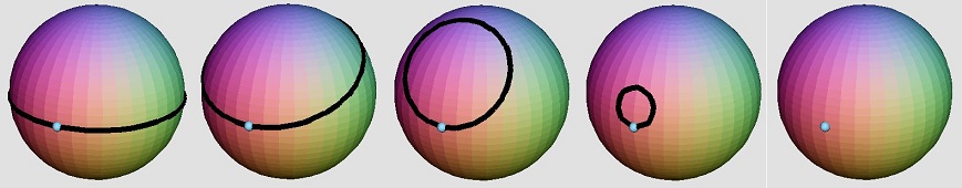
In 1904 the French mathematician Henri Poincaré asked if the three dimensional sphere is characterized as the unique simply connected three manifold. This question, the Poincaré conjecture, was a special case of Thurston's geometrization conjecture.
Perelman's proof tells us that every three manifold is built from a set of standard pieces, each with one of eight well-understood geometries _([ClayMath Institute](https://www.claymath.org/millennium-problems/poincar%C3%A9-conjecture))_.
More generally, the central problem is to determine when an equation in n-dimensional space has solutions. However at this point, we finaly found that the prime distribution has something to do with the subclasses of rank and crank partitions.

p r i m e s
1 0 0 0 0 0
2 1 0 0 0 1
3 2 0 1 0 2
4 3 1 1 0 3
5 5 2 1 0 5
6 7 3 1 0 7
7 11 4 1 0 11
8 13 5 1 0 13
9 17 0 1 1 17 ◄--- has a total of 18-7 = 11 composite √
10 19 1 1 1 ∆1 ◄--- 0th ∆prime ◄--- Fibonacci Index #18
-----
11 23 2 1 1 ∆2 ◄--- 1st ∆prime ◄--- Fibonacci Index #19
12 29 2 -1 1 ∆3 ◄--- 2nd ∆prime ◄--- Fibonacci Index #20
13 31 1 -1 1 ∆4
14 37 1 1 1 ∆5 ◄--- 3th ∆prime ◄--- Fibonacci Index #21
15 41 2 1 1 ∆6
16 43 3 1 1 ∆7 ◄--- 4th ∆prime ◄--- Fibonacci Index #22
17 47 4 1 1 ∆8
18 53 4 -1 1 ∆9
19 59 4 1 1 ∆10
20 61 5 1 1 ∆11 ◄--- 5th ∆prime ◄--- Fibonacci Index #23
21 67 5 -1 1 ∆12
22 71 4 -1 1 ∆13 ◄--- 6th ∆prime ◄--- Fibonacci Index #24
23 73 3 -1 1 ∆14
24 79 3 1 1 ∆15
25 83 4 1 1 ∆16
26 89 4 -1 1 ∆17 ◄--- 7th ∆prime ◄--- Fibonacci Index #25
27 97 3 -1 1 ∆18
28 101 2 -1 1 ∆19 ◄--- 8th ∆prime ◄--- Fibonacci Index #26
29 103 1 -1 1 ∆20
30 107 0 -1 1 ∆21
31 109 5 -1 0 ∆22
32 113 4 -1 0 ∆23 ◄--- 9th ∆prime ◄--- Fibonacci Index #27
33 127 3 -1 0 ∆24
34 131 2 -1 0 ∆25
35 137 2 1 0 ∆26
36 139 3 1 0 ∆27
37 149 4 1 0 ∆28
38 151 5 1 0 ∆29 ◄--- 10th ∆prime  ◄--- Fibonacci Index #28
39 157 5 -1 0 ∆30
40 163 5 1 0 ∆31 ◄--- 11th ∆prime ◄--- Fibonacci Index #29
-----
41 167 0 1 1 ∆0
42 173 0 -1 1 ∆1
43 179 0 1 1 ∆2 ◄--- ∆∆1
44 181 1 1 1 ∆3 ◄--- ∆∆2 ◄--- 1st ∆∆prime ◄--- Fibonacci Index #30
45 191 2 1 1 ∆4
46 193 3 1 1 ∆5 ◄--- ∆∆3 ◄--- 2nd ∆∆prime ◄--- Fibonacci Index #31
47 197 4 1 1 ∆6
48 199 5 1 1 ∆7 ◄--- ∆∆4
49 211 5 -1 1 ∆8
50 223 5 1 1 ∆9
51 227 0 1 2 ∆10
52 229 1 1 2 ∆11 ◄--- ∆∆5 ◄--- 3rd ∆∆prime ◄--- Fibonacci Index #32
53 233 2 1 2 ∆12
54 239 2 -1 2 ∆13 ◄--- ∆∆6
55 241 1 -1 2 ∆14
56 251 0 -1 2 ∆15
57 257 0 1 2 ∆16
58 263 0 -1 2 ∆17 ◄--- ∆∆7 ◄--- 4th ∆∆prime ◄--- Fibonacci Index #33
59 269 0 1 2 ∆18
60 271 1 1 2 ∆19 ◄--- ∆∆8
61 277 1 -1 2 ∆20
62 281 0 -1 2 ∆21
63 283 5 -1 1 ∆22
64 293 4 -1 1 ∆23 ◄--- ∆∆9
65 307 3 -1 1 ∆24
66 311 2 -1 1 ∆25
67 313 1 -1 1 ∆26
68 317 0 -1 1 ∆27
69 331 5 -1 0 ∆28
70 337 5 1 0 ∆29 ◄--- ∆∆10
71 347 0 1 1 ∆30
72 349 1 1 1 ∆31 ◄--- ∆∆11 ◄--- 5th ∆∆prime ◄--- Fibonacci Index #34
73 353 2 1 1 ∆32
74 359 2 -1 1 ∆33
75 367 1 -1 1 ∆34
76 373 1 1 1 ∆35
77 379 1 -1 1 ∆36
78 383 0 -1 1 ∆37 ◄--- ∆∆12
79 389 0 1 1 ∆38
80 397 1 1 1 ∆39
81 401 2 1 1 ∆40
82 409 3 1 1 ∆41 ◄--- ∆∆13 ◄--- 6th ∆∆prime ◄--- Fibonacci Index #35
83 419 4 1 1 ∆42
84 421 5 1 1 ∆43 ◄--- ∆∆14
85 431 0 1 2 ∆44
86 433 1 1 2 ∆45
87 439 1 -1 2 ∆46
88 443 0 -1 2 ∆47 ◄--- ∆∆15
89 449 0 1 2 ∆48
90 457 1 1 2 ∆49
91 461 2 1 2 ∆50
92 463 3 1 2 ∆51
93 467 4 1 2 ∆52
94 479 4 -1 2 ∆53 ◄--- ∆∆16
95 487 3 -1 2 ∆54
96 491 2 -1 2 ∆55
97 499 1 -1 2 ∆56
98 503 0 -1 2 ∆57
99 509 0 1 2 ∆58
100 521 0 -1 2 ∆59 ◄--- ∆∆17 ◄--- 7th ∆∆prime ◄--- Fibonacci Index #36
-----
101 523 5 -1 1 ∆2 ◄--- ∆∆18 ◄--- 1st ∆∆∆prime ◄--- Fibonacci Index #37 √
102 541 5 1 1 ∆3 ◄--- ∆∆∆1 ◄--- 1st ÷÷÷composite ◄--- Index #(37+2)=#39 √
103 547 5 -1 1 ∆4
104 557 4 -1 1 ∆5 ◄--- ∆∆∆2 ◄---2nd ∆∆∆prime √
105 563 4 1 1 ∆6
106 569 4 -1 1 ∆7 ◄--- ∆∆∆3 ◄--- 3rd ∆∆∆prime √
107 571 3 -1 1 ∆8
108 577 3 1 1 ∆9
109 587 4 1 1 ∆10
110 593 4 -1 1 ∆11 ◄--- ∆∆∆4 ◄--- 2nd ÷÷÷composite ◄--- Index #(37+3)=#40 √
111 599 4 1 1 ∆12
112 601 5 1 1 ∆13 ◄--- ∆∆∆5 ◄--- 4th ∆∆∆prime √
113 607 5 -1 1 ∆14
114 613 5 1 1 ∆15
115 617 0 1 2 ∆16
116 619 1 1 2 ∆17 ◄--- ∆∆∆6 ◄--- 3rd ÷÷÷composite ◄--- Index #(37+5)=#42 √
117 631 1 -1 2 ∆18
118 641 0 -1 2 ∆19 ◄--- ∆∆∆7 ◄--- 5th ∆∆∆prime √
119 643 5 -1 1 ∆20
120 647 4 -1 1 ∆21
121 653 4 1 1 ∆22
122 659 4 -1 1 ∆23 ◄--- ∆∆∆8 ◄--- 4th ÷÷÷composite ◄--- Index #(37+7)=#44 √
123 661 3 -1 1 ∆24
124 673 3 1 1 ∆25
125 677 4 1 1 ∆26
126 683 4 -1 1 ∆27
127 691 3 -1 1 ∆28
128 701 2 -1 1 ∆29 ◄--- ∆∆∆9 ◄--- 5th ÷÷÷composite ◄--- Index #(37+11)=#48 √
129 709 1 -1 1 ∆30
130 719 0 -1 1 ∆31 ◄--- ∆∆∆10 ◄--- 6th ÷÷÷composite ◄--- Index #(37+13)=#50 √
131 727 5 -1 0 ∆32
132 733 5 1 0 ∆33
133 739 5 -1 0 ∆34
134 743 4 -1 0 ∆35
135 751 3 -1 0 ∆36
136 757 3 1 0 ∆37 ◄--- ∆∆∆11 ◄--- 6th ∆∆∆prime √
137 761 4 1 0 ∆38
138 769 5 1 0 ∆39
139 773 0 1 1 ∆40
140 787 1 1 1 ∆41 ◄--- ∆∆∆12 ◄--- 7th ÷÷÷composite ◄--- Index #(37+17)=#54 √
141 797 2 1 1 ∆42
142 809 2 -1 1 ∆43 ◄--- ∆∆∆13 ◄--- 7th ∆∆∆prime √
143 811 1 -1 1 ∆44
144 821 0 -1 1 ∆45
145 823 5 -1 0 ∆46
146 827 4 -1 0 ∆47 ◄--- ∆∆∆14 ◄--- 8th ÷÷÷composite ◄--- Index #(37+19)=#56 √
147 829 3 -1 0 ∆48
148 839 2 -1 0 ∆49
149 853 1 -1 0 ∆50
150 857 0 -1 0 ∆51
151 859 5 -1 -1 ∆52
152 863 4 -1 -1 ∆53 ◄--- ∆∆∆15 ◄--- 9th ÷÷÷composite ◄--- Index #(37+23)=#60 √
153 877 3 -1 -1 ∆54
154 881 2 -1 -1 ∆55
155 883 1 -1 -1 ∆56
156 887 0 -1 -1 ∆57
157 907 5 -1 -2 ∆58
158 911 4 -1 -2 ∆59 ◄--- ∆∆∆16 ◄--- 10th ÷÷÷composite ◄--- Index #(37+29)=#66 √
159 919 3 -1 -2 ∆60
169 929 2 -1 -2 ∆61 ◄--- ∆∆∆17 ◄--- 8th ∆∆∆prime √
161 937 1 -1 -2 ∆62
162 941 0 -1 -2 ∆63
163 947 0 1 -2 ∆64
164 953 0 -1 -2 ∆65
165 967 5 -1 -3 ∆66
166 971 4 -1 -3 ∆67 ◄--- ∆∆∆18 ◄--- 11th ÷÷÷composite ◄--- Index #(37+31)=#68 √
167 977 4 1 -3 ∆68
168 983 4 -1 -3 ∆69
169 991 3 -1 -3 ∆70
170 997 3 1 -32 ∆71 ◄--- ∆∆∆19 ◄--- 9th ∆∆∆prime √
The Ricci flow is a pde for evolving the metric tensor in a Riemannian manifold to make it rounder, in the hope that one may draw topological conclusions from the existence of such “round” metrics.
Poincaré hypothesized that if such a space has the additional property that each loop in the space can be continuously tightened to a point, then it is necessarily a three-dimensional sphere _([Wikipedia](https://en.wikipedia.org/wiki/Poincar%C3%A9_conjecture))_
The Ricci Flow method has now been developed not only in to geometric but also to the conversion of facial shapes in three (3) dimensions to computer data. A big leap in the field of AI (Artificial intelligence). No wonder now all the science leads to it.
So what we've discussed on this wiki is entirely nothing but an embodiment of this solved Poincare Conjecture. This is the one placed with id: 10 (ten) which stands as the basic algorithm of π(10)=(2,3,5,7).
Many relevant topics, such as trustworthiness, explainability, and ethics are characterized by implicit anthropocentric and anthropomorphistic conceptions and, for instance, the pursuit of human-like intelligence. AI is one of the most debated subjects of today and there seems little common understanding concerning the differences and similarities of human intelligence and artificial intelligence _([Human vs AI](https://www.frontiersin.org/articles/10.3389/frai.2021.622364/full))_.
Finite collections of objects are considered 0-dimensional. Objects that are "dragged" versions of zero-dimensional objects are then called one-dimensional. Similarly, objects which are dragged one-dimensional objects are two-dimensional, and so on.
The basic ideas leading up to this result (including the dimension invariance theorem, domain invariance theorem, and Lebesgue covering dimension) were developed by **Poincaré**, Brouwer, Lebesgue, Urysohn, and Menger _([MathWorld](https://mathworld.wolfram.com/Dimension.html))_.

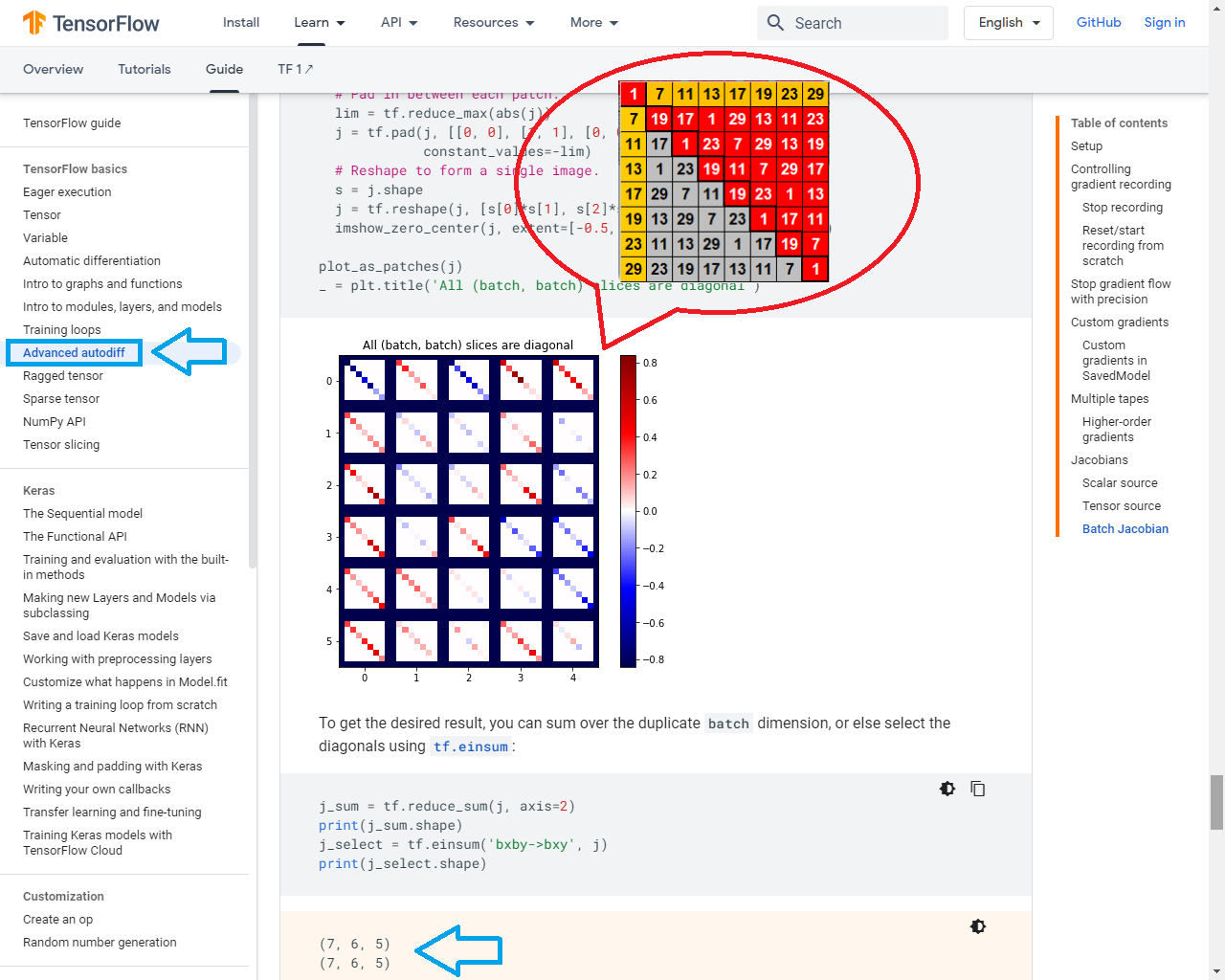
In vector calculus, the Jacobian matrix of a vector-valued function of several variables is the matrix of all its first-order partial derivatives.
It's possible to build a _[Hessian matrix](https://en.wikipedia.org/wiki/Hessian_matrix)_ for a _[Newton's method](https://en.wikipedia.org/wiki/Newton%27s_method_in_optimization)_ step using the Jacobian method. ***You would first flatten out its axes into a matrix, and flatten out the gradient into a vector.*** _([Tensorflow](https://www.tensorflow.org/guide/advanced_autodiff#batch_jacobian))_
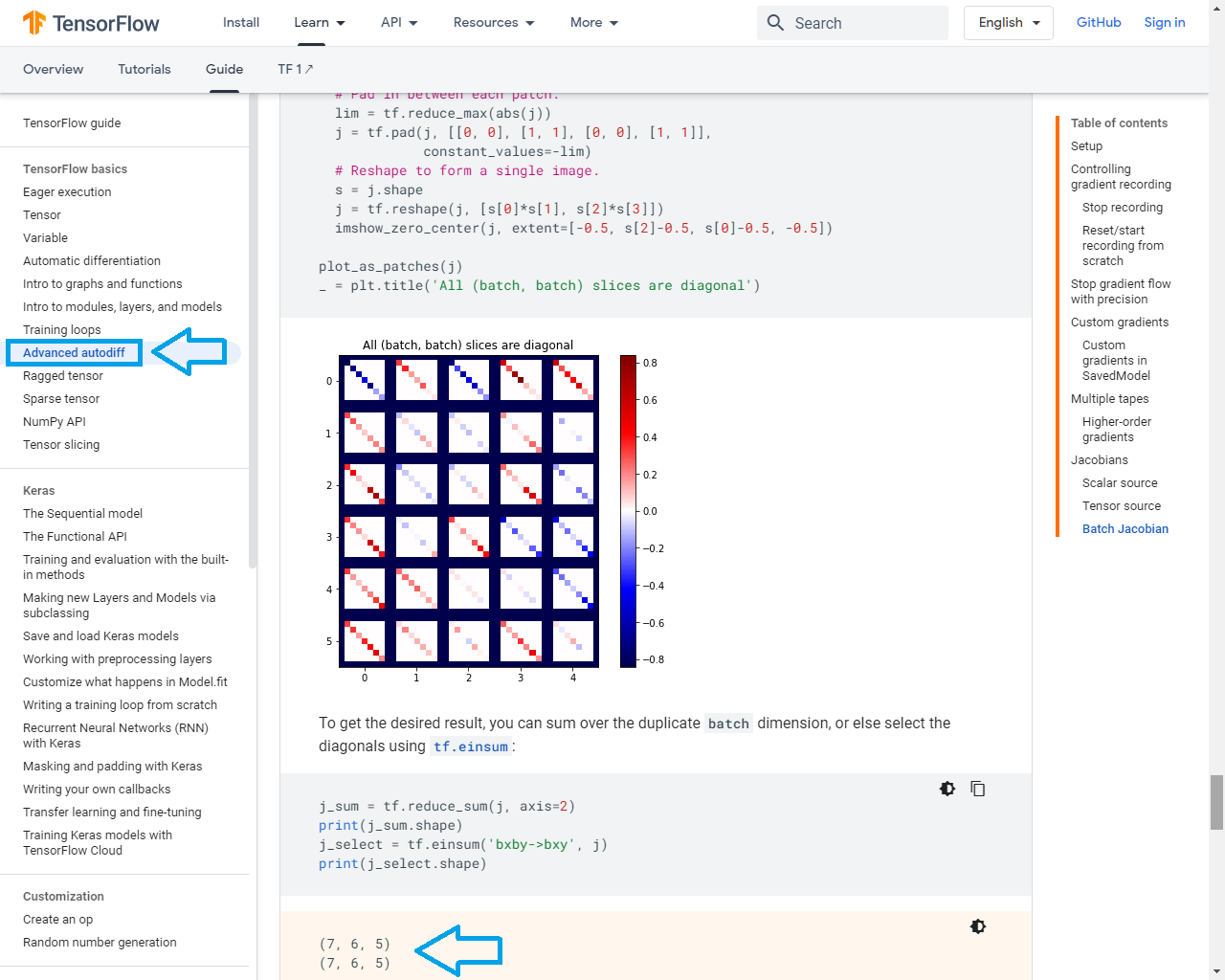
When the subclasses of partitions are flatten out into a matrix, you want to take the Jacobian of each of a stack of targets with respect to a stack of sources, where the Jacobians for each target-source pair are independent.
***When this matrix is square, that is, when the function takes the same number of variables as input as the number of vector components of its output, its determinant is referred to as the Jacobian determinant***. Both the matrix and (if applicable) the determinant ad often referred to simply as the Jacobian in literature. _([Wikipedia](https://en.wikipedia.org/wiki/Jacobian_matrix_and_determinant))_
Here we adopt an analysis of variance called N/P-Integration that was applied to find the best set of environmental variables that describe the density out of distance matrices.
With collaborators, we regularly work on projects where we want to understand the taxonomic and functional diversity of microbial community in the context of metadata often recorded under specific hypotheses. Integrating (***N-/P- integration***; see figure below) these datasets require a fair deal of multivariate statistical analysis for which I have shared the [code](https://userweb.eng.gla.ac.uk/umer.ijaz/bioinformatics/ecological.html) on this website. _([Umer.Ijaz](https://userweb.eng.gla.ac.uk/umer.ijaz/#intro))_

It can be used to build parsers/compilers/interpreters for various use cases ranging from simple config files to full fledged programming languages.
With theoretical foundations in [Information Engineering](https://en.wikipedia.org/wiki/Information_engineering) (Discrete Mathematics, Control Theory, System Theory, Information Theory, and Statistics), my research has delivered a suite of systems and products that has allowed me to carve out a niche within an extensive collaborative network (>200 academics). _([Umer.Ijaz](https://userweb.eng.gla.ac.uk/umer.ijaz/#intro))_

Since such interactions result in a change in momentum, they can give rise to classical Newtonian forces of rotation and revolution by means of orbital structure.

As you can see on the left sidebar (dekstop mode) a total of 102 items will be reached by the end of Id: 35.

So when they transfered to Id: 36 it will cover 11 x 6 = 66 items thus the total will be 102 + 66 = 168
Scheme 13:9
===========
(1){1}-7:   7'
(1){8}-13:  6‘
(1)14-{19}: 6‘
------------- 6+6 -------
(2)20-24:   5'           |
(2)25-{29}: 5'           |
------------  5+5 -------
(3)30-36:   7:{70,30,10²}|
------------             |
(4)37-48:   12• ---      |
(5)49-59:   11°    |     |
            --}30° 30•   |
(6)60-78:   19°    |     |
(7)79-96:   18• ---      |
--------------           |
(8)97-109:  13           |
(9)110-139:{30}=5x6 <--x-
            --
           {43}
The True Prime Pairs:
(5,7), (11,13), (17,19)

|-------------------------------- 2x96 -------------------------------|
|--------------- 7¤ ---------------|------------ 7¤ ------------------|
|-------------- {89} --------------|{12}|-- {30} -|-- {36} -|-- {25} -|
+----+----+----+----+----+----+----+----+----+----+----+----+----+----+
|  5 |  7 | 11 |{13}| 17 | 19 | 17 |{12}| 11 | 19 | 18 | 18 | 12 | 13 |
+----+----+----+----+----+----+----+----+----+----+----+----+----+----+
|--------- {53} ---------|---- {48} ----|---- {48} ----|---- {43} ----|
|---------- 5¤ ----------|------------ {96} -----------|----- 3¤ -----|
|-------- Bosons --------|---------- Fermions ---------|-- Gravitons--|
13 variations 48 variations 11 variations 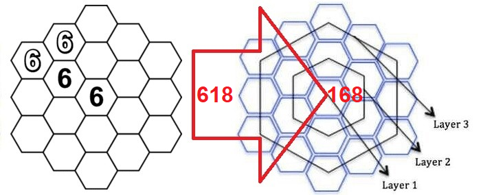
The Prime Recycling ζ(s):
(2,3), (29,89), (36,68), (72,42), (100,50), (2,3), (29,89), ...**infinity**

----------------------+-----+-----+-----+                                    ---
     7 --------- 1,2:1|   1 |  30 |  40 | 71 (2,3) ‹-------------@----        |
     |                +-----+-----+-----+-----+                        |      |
     |  8 ‹------  3:2|   1 |  30 |  40 |  90 | 161 (7) ‹---           |      5¨  encapsulation
     |  |             +-----+-----+-----+-----+             |          |      |
     |  |  6 ‹-- 4,6:3|   1 |  30 | 200 | 231 (10,11,12) ‹--|---       |      |
     |  |  |          +-----+-----+-----+-----+             |   |      |     ---
      --|--|-----» 7:4|   1 |  30 |  40 | 200 | 271 (13) --›    | {5®} |      |
        |  |          +-----+-----+-----+-----+                 |      |      |
         --|---› 8,9:5|   1 |  30 | 200 | 231 (14,15) ---------›       |      7¨  abstraction
289        |          +-----+-----+-----+-----+-----+                  |      |
 |          ----› 10:6|  20 |   5 |  10 |  70 |  90 | 195 (19) --› Φ   | {6®} |
  --------------------+-----+-----+-----+-----+-----+                  |     ---
     67 --------› 11:7|   5 |   9 |  14 (20) --------› ¤               |      |
     |                +-----+-----+-----+                              |      |
     |  78 ‹----- 12:8|   9 |  60 |  40 | 109 (26) «------------       |     11¨  polymorphism
     |  |             +-----+-----+-----+                       |      |      |
     |  |  86‹--- 13:9|   9 |  60 |  69 (27) «-- 3xΔ9 (2xMEC30) | {2®} |      |
     |  |  |          +-----+-----+-----+                       |      |     ---
     |  |   ---› 14:10|   9 |  60 |  40 | 109 (28) -------------       |      |
     |  |             +-----+-----+-----+                              |      |
     |   ---› 15,18:11|   1 |  30 |  40 | 71 (29,30,31,32) ----------        13¨  inheritance
329  |                +-----+-----+-----+                                     |
  |   ‹--------- 19:12|  10 |  60 | {70} (36) ‹--------------------- Φ        |
   -------------------+-----+-----+                                          ---
    786 ‹------- 20:13|  90 |  90 (38) ‹-------------- ¤                      |
     |                +-----+-----+                                           |
     | 618 ‹- 21,22:14|   8 |  40 |  48 (40,41) ‹----------------------      17¨  class
     |  |             +-----+-----+-----+-----+-----+                  |      |
     |  | 594 ‹- 23:15|   8 |  40 |  70 |  60 | 100 | 278 (42) «--     |{6'®} |
     |  |  |          +-----+-----+-----+-----+-----+             |    |     ---
      --|--|-»24,27:16|   8 |  40 |  48 (43,44,45,46) ------------|----       |
        |  |          +-----+-----+                               |           |
         --|---› 28:17| 100 | {100} (50) ------------------------»           19¨  object
168        |          +-----+                                                 |
|         102 -› 29:18| 50  | 50(68) ---------> ∆27-∆9=Δ18                    |
----------------------+-----+                                                ---