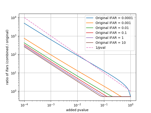
pvalue combining tests

Test combining pvalues from 1) the 2-ifo time slide background estimate 2) the 3+-ifo SNR time series followup, using the Fisher method given a nominal analysis time.

Outcome of combining and maximizing

Procedure followed:

1. Convert 2-ifo coinc IFAR to p-value (p1) using a notional livetime (eg 0.001yr ~ 9 hours)
2. Combine p1 with p-value resulting from 3rd ifo SNR time series (p2) via Fisher method
3. Convert this combined p-value back to IFAR
4. Take the maximum of this combined IFAR and the original 2-ifo IFAR to avoid any event being made much less significant by 'followup', apply trials factor of 2 to the result.

import numpy, pylab
from scipy.stats import combine_pvalues

def ftop(f, ft):
    # calculates p-value corresponding to FAR 'f' and foreground time 'ft'
    return 1 - numpy.exp(-ft * f)

def ptof(p, ft):
    # calculates FAR corresponding to p-value 'p' and foreground time 'ft'
    return numpy.log(1.0-p) / -ft

# use a fixed notional livetime to do conversions
ftime = 0.001
# IFAR from 2-ifo coinc background estimate
ifars = [0.0001, 0.001, 0.01, 0.1, 1, 10]
# 'added' p-values resulting from 3rd (etc.) ifo followup
pvalues = numpy.logspace(-4, 0, num=50)

for ifar in ifars:
    # p-value from 2-ifo coinc IFAR
    p1 = ftop(1.0/ifar, ftime)

    # Fisher combination
    cp = numpy.array([combine_pvalues([p1, p2])[1] for p2 in pvalues])

    # new IFAR
    nifar = 1.0 / ptof(cp, ftime)

    # combine with original & take trials factor
    mifar = numpy.maximum(ifar, nifar) / 2.0

    pylab.plot(pvalues, mifar / ifar, label='Original IFAR = %s' % ifar)

pylab.plot(pvalues, 1.0/pvalues, linestyle='--', label='1/pval')
pylab.grid()
pylab.xscale('log')
pylab.yscale('log')
pylab.ylabel('ratio of ifars (combined / original)')
pylab.xlabel('added pvalue')
pylab.legend()
pylab.savefig('farchange_0p1_max.png')

Checking consistency

Here we do a Monte Carlo study of the consistency of the 'p-value combination' procedure above. There are two parameters to consider: the rate of events for which this 'followup' is done, and the notional livetime ftime used to convert (I)FAR to p-value and back. We describe the event rate via the waiting time wt to next event.

We will find that

1. If the notional/conversional livetime ftime >> inverse event rate wt, the 'combined' IFAR is not consistent; too many false alarms are produced.
2. If ftime << wt the 'combined' IFAR is over-conservative, too few false alarms.
3. If ftime == wt the 'combined' IFAR is consistent or marginally conservative.
4. If ftime = k wt for about 1<k<5, the 'combined IFAR' is still consistent. I.e. the conversion livetime may be somewhat larger than the inverse event rate without problems emerging.

The script below compares (1) the original IFARs, (2) p-value combination via Fisher method with livetime = waiting time to next event (3) p-value combination via Fisher method with a different, fixed reference time, and (4) taking the max of combination IFAR with-fixed-reference-time and original IFAR, with trials factor 2. We will consider a basic event rate of 10^4 per year, i.e. wt just below 1 hour. (We also make a plot for a rate 10^3 per year as an illustrative case.)

import numpy, pylab
from scipy.stats import combine_pvalues
from numpy.random import uniform
from numpy.random import seed
#seed(0)

def ptof(p, ft):
   return numpy.log(1.0 - p) / -ft

def ftop(f, ft):
   return 1 - numpy.exp(-ft * f)

def fisher_combine(p, q):
    combvals = [combine_pvalues([v1, v2], method='fisher')[1] for v1, v2 in zip(p, q)]
    return numpy.array(combvals)

size = 500000

# p1 represents 'original' result from 2-ifo bg
p1 = uniform(0, 1, size=size)
# p2 represents 3- or 3+n-ifo followup
p2 = uniform(0, 1, size=size)

print 'Combining with Fisher'
# combine (implicitly using actual livetime)
cp = fisher_combine(p1, p2)

wt = 0.0001  # actual (average) waiting time between events
# 0.1yr is a bit over a month
# 0.01yr ~ 3.7 days
# 0.001yr ~ 8.7h
# 0.0001yr ~ 52min
# 0.00001yr ~ 5.2min
btime = wt * size  # total time over all random trials

# 'ifars' is original 2-ifo IFAR
ifars = 1.0 / ptof(p1, wt)
cifars = 1.0 / ptof(cp, wt)

# define cumulative rate to plot as y-axis for sorted output IFAR values
crate = numpy.arange(size, 0, -1) / btime

print 'Scaling and combining'

fixedlt = True
if fixedlt:
    # first method uses a fixed notional livetime
    ftime = 0.0005
    # convert original FARs to notional p-values
    p3 = ftop(1.0 / ifars, ftime)
    cp2 = fisher_combine(p3, p2)
    sifar = 1.0 / ptof(cp2, ftime)
else:
    # new 'scaling' method uses notional livetime of fac * 2-ifo IFAR
    # the p-value corresponding to this is always 1 - exp(-fac)
    # so calculate it for e.g. IFAR = foreground time
    ifarfac = 0.02
    ftime = ifarfac * ifars
    # dummy IFAR value
    p3 = ftop(1./wt, ifarfac * wt)
    cp2 = fisher_combine(p3 * numpy.ones_like(p2), p2)
    sifar = 1.0 / ptof(cp2, ftime)

# maximize between original and adjusted IFAR and add trials factor
mifars = numpy.maximum(ifars, sifar) / 2.0

ifars.sort()
cifars.sort()
mifars.sort()
sifar.sort()

if fixedlt:
    pylab.plot(sifar, crate, label=r'combined, livetime $t=%.2g$' % lt, alpha=0.6)
else:
    pylab.plot(sifar, crate, label=r'combined, livetime $%.2g\times$IFAR$_0$' % ifarfac, alpha=0.6)
#pylab.plot(cifars, crate, label='combined (Fisher)', alpha=0.6)
pylab.plot(mifars, crate, label='max(combined,orig)/2', alpha=0.6)
pylab.plot(ifars, crate, label='orig ifars', alpha=0.6)
pylab.plot(1./crate, crate, c='k', linestyle='--', label='1/IFAR', alpha=0.4)
pylab.legend()
pylab.xscale('log')
pylab.yscale('log')
pylab.ylabel('Cumulative Rate (/yr)')
pylab.xlabel('IFAR (yr)')
pylab.savefig('combining_wait0p0001_0p0005.png')

Waiting time 0.001yr, conversion livetime 1e-4yr

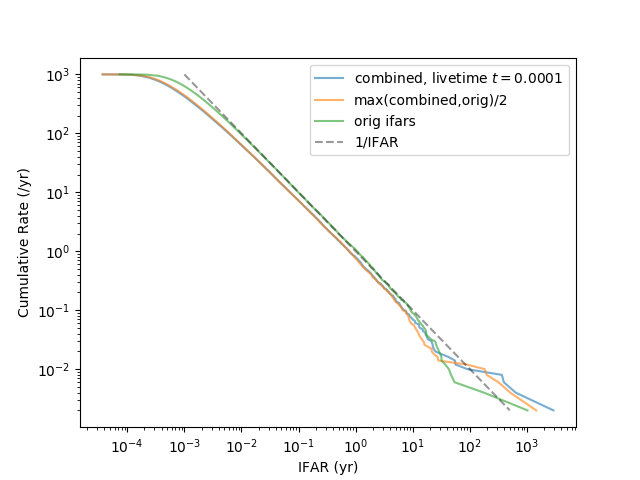
The combined-via-Fisher-method IFAR and the max-with-trials-factor IFAR are both over-conservative.

Waiting time 1e-4yr, conversion livetime 1e-4yr

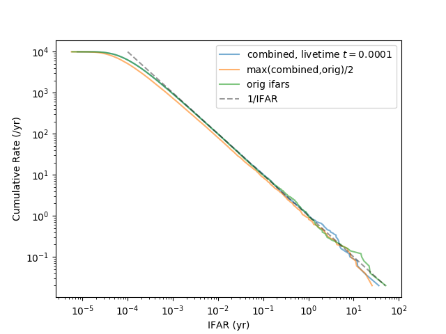
The combined-via-Fisher-method IFAR is completely consistent; the max-with-trials-factor IFAR is slightly conservative. We think this is because the combined IFAR is correlated with the original IFAR, ie they do not represent completely independent trials.

Waiting time 1e-4yr, conversion livetime 0.001yr

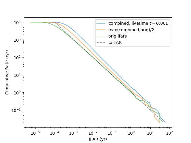
The combined-via-Fisher-method IFAR is inconsistent; the max-with-trials-factor IFAR is somewhat less inconsistent but still clearly above the 1/IFAR line.

Waiting time 1e-4yr, conversion livetime 5e-4yr

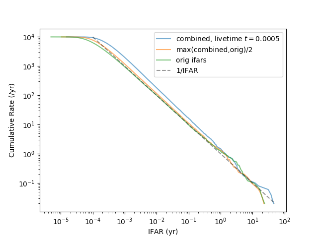
The combined-via-Fisher IFAR is slightly inconsistent (small excess of false alarms), however the max-with-trials-factor step appears to remove essentially the entire excess.