(Step 5) Path Tracing

Up to this point, your renderer simulates light which begins at a source, bounces off a surface, and hits a camera. However in the real world, light can take much more complicated paths, bouncing of many surfaces before eventually reaching the camera. Simulating this multi-bounce light is referred to as indirect illumination, and it is critical to producing realistic images, especially when specular surfaces are present. In this task you will modify your ray tracer to simulate multi-bounce light, adding support for indirect illumination.

Step 1

First, you must modify Pathtracer::trace_ray() to simulate multiple bounces. We recommend using the Russian Roulette algorithm discussed in class.

The basic structure will be as follows:

(1) Randomly select a new ray direction using BSDF::sample_f() (which you will implement in Step 2)
(2) Potentially terminate the path (using Russian roulette)
(3) Recursively trace the ray to evaluate weighted reflectance contribution due to light from this direction. Remember to respect the maximum number of bounces from ray_max_depth.

Step 2

Now, Implement BSDF::sample_f for diffuse surfaces (DiffuseBSDF:sample_f), which randomly samples from the distribution. The implementation of DiffuseBSDF::f is already provided to you, and note that there is documentation in bsdf.h.

Notes:

The class sampler.cpp contains helper functions for random sampling, which you may use if you desire. The DiffuseBSDF starter code already has a private member CosineWeightedHemisphereSampler3D sampler, but you need to implement the corresponding helper in sampler.cpp if you want to use it.
Task 6 contains further discussion of sampling BSDFs, reading ahead may help your understanding.

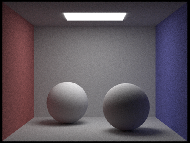
After correctly implementing diffuse BSDF and path tracing, your renderer should be able to make a beautifully lit picture of the Cornell Box with:

    ./scotty3d -s 1024 -m 4 -t 8 ../media/pathtracer/advanced/CBspheres_lambertian.dae

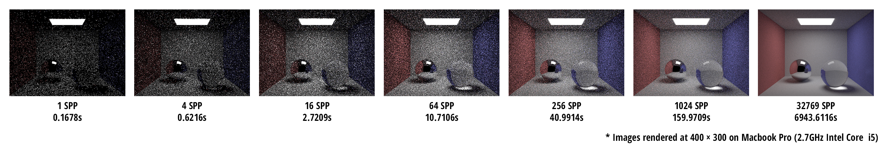
Note the time-quality tradeoff here. With these commandline arguments, your path tracer will be running with 8 worker threads at a sample rate of 1024 camera rays per pixel, with a max ray depth of 4. This will produce an image with relatively high quality but will take quite some time to render. Rendering a high quality image will take a very long time as indicated by the image sequence below, so start testing your path tracer early!

Here are a few tips:

The termination probability of paths can be determined based on the overall throughput of the path (you'll likely need to add a field to the Ray structure to implement this) or based on the value of the BSDF given wo and wi in the current step. Keep in mind that delta function BSDFs can take on values greater than one, so clamping termination probabilities derived from BSDF values to 1 is wise.
To convert a Spectrum to a termination probability, we recommend you use the luminance (overall brightness) of the Spectrum, which is available via Spectrum::illum()
We've given you some pretty good notes on how to do this part of the assignment, but it can still be tricky to get correct.