lattice_sum

Lattice sum

baptiste Auguié -- 22 June, 2014

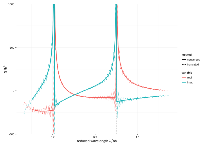
Comparison of numerical approximation to the lattice sum for a 2D array of dipoles and its converged solution.

data(G0)

## number of dipoles for the numerical evaluation
N <- 100
pitch <- 0.6
lambda0 <- seq(0.45,1.0,length=300)
n <- 1.33
lambda <- lambda0 / n
lambdap <- lambda / pitch

S1 <- array_factor(wavelength=lambda,
                   N=N, pitch=pitch)

interpolate.fun <- function(x, y){
  list(re=approxfun(x, Re(y)),
       im=approxfun(x, Im(y)))
}

gfun <- interpolate.fun(G0$wavelength, G0$Gxx)

numerical <- data.frame(lambdap = S1$wavelength / pitch,
                      real = Re(S1$S)*pitch^3,
                      imag = Im(S1$S)*pitch^3,
                      method = "truncated")

converged <- data.frame(lambdap = lambdap,
                     real = gfun$re(lambdap),
                     imag = gfun$im(lambdap),
                     method = "converged")
m <- melt(rbind(converged, numerical), id = c("lambdap", "method"))
p <- ggplot(m,
            aes(lambdap, value, colour=variable, linetype=method)) +
  geom_vline(xintercept = c(1, sqrt(2)/2), linetype=2, colour="grey")+
  geom_line() +  
  geom_path(data=subset(m, method == "converged"),size=1) + 
  coord_cartesian(ylim=c(-500, 1000)) +
  labs(x=expression("reduced wavelength "*lambda/nh), y=expression(S/h^3))

p